A method for determining a physical law using the simple pendulum as a model By name Lab Partner: name 7 September 2000 Abstract A process for determining a physical law was executed using the simple pendulum as a model. The three variables thought most likely to be major influences on pendulum period were selected. Each variable was tested while holding the others constant. Displacement affected period, but for displacements less than 10 degrees string length had the most significant effect on period. The law relating period to string length was determined. The experimental law did not agree with the accepted law within experimental uncertainty. ! 1 INTRODUCTION AND THEORY The simple pendulum system was selected to test a method for determining physical laws. The method was applied to determine which variables influence the period of the pendulum. The goal was to derive the law that relates the period of the pendulum to the most significant variables. A diagram of the simple pendulum is shown in Figure 1. {Note that I have called out the figure in the text before the figure appears.} ! Figure 1. Diagram of the simple pendulum. θ is the displacement angle, L is the length of the pendulum, g is the acceleration due to gravity, m is the mass of the pendulum bob, and T is the tension in the string. {Note: This is Figure 1, not Figure 1.1. Number your figures and tables sequentially as they appear in the text. This is a ! 2 stand-alone report, not a report in a sequence of reports in lab.} Operational definition of period: Time for pendulum to go from any point in its motion back to that same point, and traveling in the same direction. Table 1. is a list of equipment used in the experiment. {Table mentioned in text before it appears.} {I have taken care to see that the table is all on one page and does not flow to a second page.} Table 1. Equipment Used. Experimental support rod clamped to lab bench Experimental support arm fastened to support rod String Clamped on the experimental support arm ~ 1.1 m long There was a loop at one end Pendulum bobs Six different materials: cork, wood, steel, lead, aluminum, and brass All bobs had hooks to which the loop in the string was attached All bobs were the same size as observed by eye Meter stick Protractor PASCO Photogate operating in pendulum mode PASCO Model 500 Interface ! 3 Pentium computer running Windows NT Science Workshop Software Microsoft Excel {table 1 is where you describe the equipment was used. This is not the place to tell how it was used. That goes in the experimental procedure in the text.} DESCRIPTION OF THE EXPERIMENT DATA AND ANALYSIS Note to students. The nature of this experiment does not lend itself to following the FORMAT I specified in my e-mail guidance and on my web site. For the formal reports, use the guidance on the web.

1. A method for determining a physical law using the simple
pendulum as a model
By
name
Lab Partner: name
7 September 2000
Abstract
A process for determining a physical law was executed using
the simple pendulum as a
model. The three variables thought most likely to be major
influences on pendulum
period were selected. Each variable was tested while holding
the others constant.
Displacement affected period, but for displacements less than
10 degrees string length
had the most significant effect on period. The law relating
period to string length was
determined. The experimental law did not agree with the
accepted law within
experimental uncertainty.

2. ! 1
INTRODUCTION AND THEORY
The simple pendulum system was selected to test a method for
determining physical
laws. The method was applied to determine which variables
influence the period of the
pendulum. The goal was to derive the law that relates the
period of the pendulum to the
most significant variables. A diagram of the simple pendulum
is shown in Figure 1.
{Note that I have called out the figure in the text before the
figure appears.}
!
Figure 1. Diagram of the simple
pendulum. θ is the displacement angle, L is the
length of the pendulum, g is the acceleration due to
gravity, m is the mass of the pendulum bob, and T is
the tension in the string. {Note: This is Figure 1,
not Figure 1.1. Number your figures and tables

3. sequentially as they appear in the text. This is a
! 2
stand-alone report, not a report in a sequence of
reports in lab.}
Operational definition of period: Time for pendulum to go from
any point
in its motion back to that same point, and traveling in the same
direction.
Table 1. is a list of equipment used in the experiment. {Table
mentioned
in text before it appears.} {I have taken care to see that the
table is all
on one page and does not flow to a second page.}
Table 1. Equipment Used.
Experimental support rod clamped to lab bench
Experimental support arm fastened to support rod
String
Clamped on the experimental support arm
~ 1.1 m long

4. There was a loop at one end
Pendulum bobs
Six different materials: cork, wood, steel, lead, aluminum, and
brass
All bobs had hooks to which the loop in the string was attached
All bobs were the same size as observed by eye
Meter stick
Protractor
PASCO Photogate operating in pendulum mode
PASCO Model 500 Interface
! 3
Pentium computer running Windows NT
Science Workshop Software
Microsoft Excel
{table 1 is where you describe the equipment was used. This is
not the place to tell how
it was used. That goes in the experimental procedure in the
text.}
DESCRIPTION OF THE EXPERIMENT DATA AND

5. ANALYSIS
Note to students. The nature of this experiment does not lend
itself to following
the FORMAT I specified in my e-mail guidance and on my web
site. For the formal
reports, use the guidance on the web site. The lesson is that my
format does not fit all
possible experiments.
The entire class examined the simple pendulum and then
brainstormed variables that
might have an impact on the period. Table 2. is the list of
possible variables generated.
Table 2. Variables that may influence period of the simple
pendulum.
String length
Gravity
Wind from the air conditioners
Air resistance
Moisture in the air
Mass of the pendulum bob
! 4

6. Phase of the moon
Temperature of room and ball
Stretchiness of the string
Mass of the string
How far the pendulum is displaced from equilibrium
Position of the earth relative to the other planets in the solar
system
Position of the earth in relation to other stars and planetary
systems in the galaxy
The group discussion determined that while each of these may
indeed affect the period of
the pendulum, the effects of many were so small as to be
undetectable with the
instrumentation available in the lab. The next step was to
determine which of these
possible variables were related to each other. Table 3 lists the
variables seen as related.
Table 4 shows the list of variables after those dependent on
others were eliminated.
Table 3. Variables from Table 2 related to each other.
Each of the following is related to gravity

7. Gravity
Phase of the moon
Position of the earth relative to the other planets in the solar
system
Position of the earth in relation to other stars and planetary
systems in the galaxy
Each of the following is related to air resistance
Air resistance
Moisture in the air
! 5
Table 4. Final list: variables that may influence period of
pendulum.
String length
Gravity
Wind from the air conditioners
Air resistance
Mass of the pendulum bob (the weight at the end of the string)
Temperature of room and ball

8. Stretchiness of the string
Mass of the string
How far the pendulum is displaced from equilibrium
The next step was to determine which of these possible
variables could be readily
controlled in the lab. The group discussed the fact that the
wind from the air conditioners
probably had, at best, a small effect. In addition, this was
basically a binary function: the
air conditioners are on and there is a wind, or they are off and
there is no wind. While it
would be possible to design a set of experiments using a fan in a
closed room to measure
the influence of air movement on period, wind, or air
movement, is not an inherent part
of the pendulum system since it is clearly possible to operate
the pendulum in a room
with no windows, fans, or air conditioners. Thus the list was
reduced to three possible
variables that seemed intuitively reasonable and that were easily
controlled in lab. These
are shown in Table 5.
! 6

9. Table 5. List of possible variables chosen to test in the lab.
Pendulum length
Mass of the bob
How far the pendulum is displaced from equilibrium.
{This table is not appropriate for Experiment 5 or Experiment
9.}
Pendulum length was defined operationally as from the point on
the bottom of the
horizontal experimental support arm where the string was
clamped to the middle of the
bob. Pendulum displacement was defined operationally as the
angle θ shown in Figure 1.
Next a series of experiments was designed to test each of these
three variables
individually. That is, when one variable was tested the other
two variables were held
constant. There is a statistical technique known as "design of
experiments" that enables
the testing of multiple variables when it is not possible to hold
all but one variable
constant. Fortunately this process was not needed for the

10. simple pendulum system as any
two of the three variables could easily be held constant while
allowing the third to vary.
Dependence of Period on Displacement Amplitude
The first possible variable tested was: the amplitude of the
displacement of the pendulum
from equilibrium. The string was fastened to the experimental
support arm as close to the
experimental support rod as possible to minimize oscillation of
the support rod when the
pendulum swings. Each two-person lab group was assigned
different displacement
angles to test. The results were combined in a single table that
covered displacements
from 3° to 70°. Displacement was measured by placing a
protractor, flat side up, against
! 7
the bottom of the horizontal support arm. The center-mark on
the flat side of the
protractor and the corresponding 90° point on the curved side
were aligned with the
pendulum string with the pendulum at rest. One lab partner

11. held the pendulum bob, with
the string taut, at the point where the angle reading of the string
on the protractor was
equal to the prescribed displacement angle. The other lab
partner started the Science
workshop software in RECORD mode and the first partner then
released the bob.
All groups used a lead bob and a pendulum length of 80 cm.
The value of 80 cm was
chosen for convenience of construction of the pendulum and for
ease in measuring the
angle of displacement. Pendulum length was measured from the
bottom of the
experimental support arm where the string was attached to the
middle of the pendulum
bob. The lead bob, the bob with the greatest mass, was used in
an effort to minimize
possible effects of air movement and air resistance. The period
for each displacement
was measured 5 times using the photogate connected to the
Science Workshop software.
The average of these five measurements was recorded. The
Science Workshop software
recorded the raw data for each of the five periods and also

12. calculated the mean of the five
data points. The raw data taken by our lab team are shown in
Table 6. The averages of
the periods from the collective experiments were compiled and
displayed in Table 7.
! 8
!
(Note to students: These graphs were created by selecting the
tables in Excel, selecting “Copy” in Excel,
moving to Word, clicking “Edit,” selecting “Paste Special,”
selecting “Microsoft Excel Worksheet Object,”
and clicking “OK.” Once you have the spreadsheet or figure in
Word, click in it, and use the small black
squares around the border of the object to re-size it so it will fit
on the Word page. There are probably
many more, and more elegant, ways to get the tables and figures
into Word, but this was the one I got to
work for me. I would be grateful if someone would show me a
better way. The problem is getting them
down to a size that looks good in Word.)
{Note: the titles here are not appropriate for Experiment 5 or
Experiment 9. For Experiment 5, you
would use e.g., “Part 1, Case 1, Raw Data” or “Part 1, Case 1,
Calculated Values,” or “Part 1, Case 2,
Raw Data,” etc.}
The entire class examined the data and discussed the following
question: Does amplitude

13. of displacement play a significant role in determining the period
of the pendulum? The
first thing noted was: Looking at the total data, period
increases steadily with increasing
displacement amplitude and in fact varies from 1.81 seconds to
1.90 seconds as
displacement angle varies from 3º to 70º. Thus, amplitude of
displacement does
influence the period of the pendulum. The percent increase in
period, as displacement
goes from 3º to 70º, was calculated as follows. We subtracted
the smallest period in
Table 7 from the largest and divided the result by the average of
the largest and smallest
period. Multiplying by 100 converted this to percent.
Table 6: Independent Variable - Amplitude. Dependent
Variable - Period--Raw Data
Station: A Bob Material: Lead Pendulum length: 80 cm
Pendulum Amp*. (deg): 3 5
1.8090 1.811
Per- 1.8092 1.813
iod 1.8091 1.812
(sec) 1.8089 1.81
1.8093 1.814

14. Avg. 1.8091 1.812
Table 7: Independent Variable - Amplitude. Dependent
Variable - Period--Averaged from Raw Data
Bob Material: Lead Pendulum length: 80 cm
Pendulum Amp*. (deg): 3 5 7 10 15 20 25 30 35 40 45 50 55 60
65 70
Exp. Station
A P 1.8091 1.812
B e 1.812 1.8144
C r 1.8172 1.8228
D I 1.8271 1.8364
E o 1.8445 1.8548
F d 1.867 1.8854
G 1.8978 1.9301
H (sec) 1.9301 1.9445
* Amp. Is Amplitude measured with a protractor
! 9
! (1)
{Follow this format for reporting equations. Place the number
in parentheses on the
right margin.} {Use Microsoft Equation Editor to write
equations.}
This small dependence of period on displacement created a
problem in designing the rest
of the experiments. If amplitude has an influence on period,

15. then which value of
amplitude should be selected to hold constant while testing
pendulum bob mass and
string length? Further examination of the period versus
displacement data suggested that
for displacement angles of less than 10º the influence of
amplitude on period was small.
Thus, when testing the effects of pendulum bob mass and string
length, the decision was
made to keep the displacement angle below 10º.
Dependence of Period on Mass of the Pendulum Bob
The class next determined to test the effect of the mass of the
pendulum bob on the
period. A set of six different bobs were used, all (to the eye)
the same diameter. The
materials were: Aluminum, brass, cork, lead, steel, and wood.
The bobs were chosen to
be roughly the same size to minimize the effect of air resistance
(the choice had been
made to not test the effect of air resistance) on the period. Each
lab group was assigned
three different bobs to test. No effort was made to use a
particular displacement, but all

16. displacements were less than 10º. The string length was chosen
to be 80 cm. Again this
choice was made for convenience in construction of the
pendulum and for ease in
measuring the angle of displacement. The raw data for our
group are shown in Table 8.
The averages from all groups were compiled and displayed in
Table 9.
%39.5(%)100
)81.190.1(
2
1
81.190.1
=•
+
−
! 10
!
The column values for the different bob materials were
averaged. Averaging the results
from different groups was an attempt to average out errors in
experimental procedure

17. between groups. Examining the data in each column by eye, it
appeared that the spread
in the period data between groups was very small. As in the
case of amplitude, we
calculated the percent difference of the variation in period as
we changed mass.
! (2)
The small value of the percent difference suggested that the
experimental procedure was
followed uniformly by each group. The column averages for
different materials did not
show a trend in their differences as did the data for period
versus amplitude. It was
therefore determined that within the accuracy or our
measurements the period would be
treated in the experiment as not depending significantly on the
bob mass.
Dependence of Period on String Length
Table 8. Independent Variable - Material. Dependent Variable
- Period--Raw Data
Group A Pendulum Length: 80 cm Pendulum Amplitude: </=
10 deg.
Brass Cork
1.8052 1.7896

18. Per- 1.8056 1.7892
iod 1.8054 1.7895
(sec) 1.8053 1.7893
1.8055 1.7894
Avg. 1.8054 1.7894
Table 9. Independent Variable - Material. Dependent Variable
- Period--
Averaged from Raw Data
Pendulum Length: 80 cm Pendulum Amplitude: </= 10 deg
Bob Material: Aluminum Brass Cork Lead Steel Wood
Expimental Group
A P 1.8054 1.7894 1.8061
B e 1.7965 1.7881 1.8055
C r 1.7966 1.8067 1.8028
D I 1.8066 1.8025 1.7988
E o 1.8049 1.7875 1.8062
F d 1.7957 1.7895 1.806
G 1.795 1.8058 1.8021
H (sec) 1.8055 1.8018 1.8009
Period (s) (Column Ave.) 1.79595 1.80515 1.788625 1.80605
1.8023 1.79985
%96.0(%)100
)7888.180605.1(
2
1
7888.180605.1
=∗

19. −
−
! 11
Finally, the effect of string length on period was examined.
Displacements were less than
10º. Lead was chosen as the pendulum bob material to
minimize the impact of air
resistance. Each group was assigned three string lengths.
String length was, as noted
above, measured from the center of the pendulum bob to the
bottom of the horizontal
experimental support bar. The raw data for out group are shown
in Table 10 while the
data and averages from all groups were compiled and displayed
in Table 11.
!
Examining the data in Table 11, it is clear that period increases
steadily with increasing
pendulum length by approximately a factor of three as one goes
from a length of 10 cm to
one of 100 cm. As above, we calculated the percent difference

20. as follows.
! (3)
This is a far larger dependence of period on pendulum length
than the dependence that
was observed on amplitude where the percent difference was
5.39% in going from a
displacement of 3º to one of 70º. Clearly, of the three variables
examined, pendulum
length has the greatest impact on period of the pendulum.
Table 10: Independent Variable - Length. Dependent Variable
- Period--Raw Data
Group: A Bob Material: Lead Pendulum Amplitude: </= 10
deg
Pend. Length (cm) 10 15 20
0.6588 0.7894 0.9007
Per- 0.6589 0.7888 0.9005
iod 0.6587 0.7891 0.9008
(sec) 0.6586 0.7892 0.9004
0.659 0.789 0.9006
Avg. 0.6588 0.7891 0.9006
Table 11: Independent Variable - Length. Dependent Variable
- Period--Averaged from Raw Data
Bob Material: Lead Pendulum Amplitude: </= 10 deg
Pendulum Length (cm):
Exp. Station 10 15 20 25 30 35 40 45 55 60 65 70 75 80 85 90

21. 95 100
A P 0.6588 0.7891 0.9006
B e 0.9013 0.9994 1.0993
C r 1.0962 1.1901 1.2751
D I 1.2762 1.3459 1.4868
E o 1.4846 1.5544 1.6152
F d 1.6143 1.6846 1.7499
G 1.7496 1.8019 1.8539
H (sec) 1.9166 1.9179 1.923
Period (s) Col. Avg. 0.6588 0.7891 0.9010 0.9994 1.0978
1.1901 1.2757 1.3459 1.4857 1.5544 1.6148 1.6846 1.7498
1.8019 1.8539 1.9166 1.9179 1.9230
%93.97(%)100
)6588.09230.1(
2
1
6588.09230.1
=•
−
−
! 12
At this point, the class had concluded that, for displacement
amplitudes of less than 10º,
the primary influence on period, of the three variables selected
to test, was pendulum

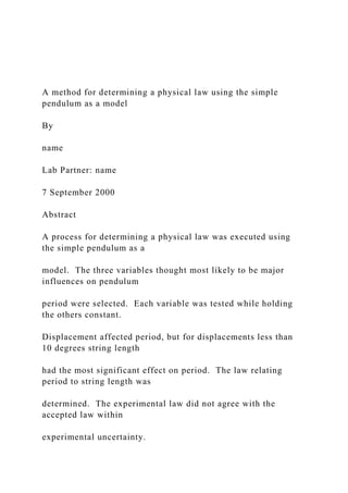
22. length. It was now necessary to determine the law that related
period and pendulum
length. The data on period and pendulum length from Table 11
were entered into
columns in Excel (See Table 12.) and Excel was used to graph
period versus pendulum
length (See Figure 2.).
! !
Figure 2.
Figure 2, the graph of the measured periods versus the measured
pendulum lengths, is
curved. Had it been straight, it would have been possible to
calculate the slope and, to
use Eqn. (4), the equation of a straight line,
Y = mX + b (4)
to determine the functional relationship between period and
pendulum length (the law
that relates the two variables). In Eqn. (4), m is the slope, and
b is the y-intercept (the
Table 12: Data for analysis of
period versus string length
String Sqrt of Best Fit

23. Length Period Length Period
(cm) (s) (cm^1/2) (s)
10 0.659 3.162 0.649
15 0.789 3.873 0.789
20 0.901 4.472 0.907
25 0.999 5.000 1.011
30 1.098 5.477 1.105
35 1.190 5.916 1.192
40 1.276 6.325 1.272
45 1.346 6.708 1.348
55 1.486 7.416 1.487
60 1.554 7.746 1.552
65 1.615 8.062 1.615
70 1.685 8.367 1.675
75 1.750 8.660 1.733
80 1.802 8.944 1.789
85 1.854 9.220 1.843
90 1.917 9.487 1.896
95 1.918 9.747 1.947
100 1.970 10.000 1.997
Actual Data for Lead Ball
Pendulum
with Amplitude <10 Degrees
P
er
io
d
(s
)

24. 0.5
0.9
1.4
1.8
2.3
Length (cm)
10 33 55 78 100
! 13
vertical axis value where the line crosses the vertical axis). In
this case, if the line had
been straight, the equation would have been Eqn. (5)
T = mL + b (5)
where T is period, and L is string length. There are curve-
fitting programs that will
determine the functional relationship from the raw data, but a
potentially easier way was
selected. If a simple transformation of one of the variables
could be found that, when
plotted against the other, untransformed variable, yielded a
straight line, Eqn. (5) could

25. then be used to write Eqn. (6) (for example) for the new line.
T = m(transformation of L) + b (6)
Functional behaviors common to physical laws include: Square
(quadratic), square root,
and exponential. The class noted that it seems physically
reasonable that if the length of
the pendulum goes to zero then the period should also be zero.
It was noted that the
linear equation and the exponential equation did not satisfy this
physical condition and
thus could be discarded as possibilities. This left square and
square root dependence. By
inspection, the graph seemed to resemble a square root function.
Thus the choice was
made to try taking the square root of string length and plotting
period versus square root
of string length. The square roots of the string lengths were
calculated using Excel and
the results are shown in Table 12. The graph of period versus
square root of string length
is shown in Figure 3. (Note: Initially only points were
! 14

26. !
Figure 3.
graphed. The line was added later using the technique
described below.) The graph
appeared to be a straight line. To test this, Excel was used to
do a regression analysis of
the data. A regression analysis is a technique for fitting the
best straight line to a set of
data points. The results are shown in Table 13. The value of R
Square in the regression
output is approximately .999 (See Table 13.). The closer this
number is to 1, the better
the data fit a straight line. The R Square value of .999 from the
regression analysis
indicated that the data could be represented very accurately by a
straight line. Thus it was
concluded that the correct functional relationship between
period (T) and string length
(L) is represented by Eqn. (7)
T ∝ L1/2 (7)
Slope (0.1971) and y-intercept (.0258) from the regression
analysis (See Table 13.) were

27. used to construct a line through the data. A new column in
Table 12 was created entitled
“Best Fit Period (s).” This column was the best-fit period
calculated by Eqn. (8)
Analysis of Lead Ball Pendulum w/ Best
Fit Line from Regression
P
er
io
d
(s
)
0.5
0.8
1.1
1.5
1.8
2.1
String Length1/2 (cm)1/2
3.0 4.4 5.8 7.2 8.6 10.0
y = 0.1967x + 0.0297
! 15

28. !
Tbest fit = 0.1971 L1/2 + 0.0258 (8)
Excel was used to place the line (without points) over the points
from the measurements
(points but no line) to generate the graph shown in Figure 3.
Eqn. (8) is our experimental
law that gives period as a function of pendulum length.
RESULTS
The accepted law for period versus pendulum length for small
amplitudes is Eqn. (9)
! (9)
or
! (10)
Eqn. (11) gives the percent difference between the experimental
and theoretical slope.
Percent Difference = [(measured – accepted)/accepted] x 100
(11)
or
Percent Difference = ! (12)

29. Percent uncertainty in the slope (See Table 13.) in Eqn. (8) was
found using Eqn. (13)
Percent uncertainty = [(uncertainty in slope)/slope] x 100(%)
(13)
or
Table 13. Regression analysis output
Regression Statistics
R Square 0.998976243
Coefficients Standard Error
Intercept 0.025838749 0.011727393
X Variable 1 0.197090312 0.001577343
g
L
T π2=
LT 201.0=
%94.1(%)100
201.0
201.01971.0
−=•
−
! 16

30. Percent uncertainty = ! (14)
Since the percent uncertainty in the measured value for the
constant in Eqn. (8) is smaller
than the percent difference between measured and accepted
values of the constant, the
measured results do not agree with the accepted answer. This
can be seen in another way
by comparing the range of the measured value of the constant
(0.19709 ± 0.00158—
0.19551 to 0.19867) to the accepted value (0.2007—for which
no uncertainty range is
available). The accepted value does not fall within the
uncertainty range of the measured
result and again we see that the result does not agree with the
accepted value.
Another indication that something is amiss with the
experimental results is that the
accepted formula does not have a value for the y-intercept. The
value for the intercept
with its uncertainty, as determined by the regression analysis
(See Table 13.), was
y-intercept = 0.0258 ± 0.0117 (15)
The uncertainty range for the y-intercept (given as “Standard
Error” in the regression)

31. does not contain zero, so within experimental uncertainty, the
results are not consistent
with a y-intercept of zero. If the string length is zero one would
expect the period to be
zero also. Thus the fact that Eqn. (8) has a non-zero value for
the y-intercept indicates
experimental error.
Two possible sources of the error in the experiment were
identified.
%0080.0(%)100
19709.0
00158.0
=•
! 17
1. There is a small dependence of period on displacement that
was not taken into
consideration. To take amplitude into account, the accepted
law, Eqn. (16) , could be 1
used.
! (16)
where g is the acceleration due to gravity and Θ is the angle of

32. displacement of the
pendulum from equilibrium.
For a displacement angle of 15º, the correction factor to Eqn.
(8) is less than 0.5%1. If we
multiply the slope from the regression (0.1971 from Eqn. (8))
by 0.005 (.5%) we get
0.1971 x 0.005 = 0.0010 (17)
Adding this result to .1971 and recalculating the percent
difference in Eqn. 12, one finds
! (18)
Comparing this to the percent uncertainty in Eqn. 14, it is clear
percent uncertainty is still
smaller than the absolute value of the percent difference. Thus
even with this correction
our results do not agree with the accepted equation for the
simple pendulum.
2. The dip in the curve at large values of string length shows
clearly in the period
versus string length plot in Figure 2. Similarly, the best-fit line
does not follow the points
as closely at large pendulum lengths as at smaller lengths for
the data on period versus
square root of pendulum length in Figure 3. The data for large

33. pendulum lengths should
be taken again and greater care used in measuring the pendulum
length from the middle
⎟
⎟
⎠
⎞
⎜
⎜
⎝
⎛
+
Θ
⎟
⎠
⎞
⎜
⎝
⎛
⎟
⎠
⎞
⎜
⎝
⎛
+

34. Θ
⎟
⎠
⎞
⎜
⎝
⎛
+= ...
2
sin
4
3
2
1
2
sin
2
1
12 4
22
2
2
g
L
T π

35. %443.1(%)100
201.0
201.01981.0
−=•
−
University Physics, by Hugh D. Young, 8th Ed., Adison-
Wesley, 1992, p. 361.1
! 18
of the pendulum bob to the bottom of the horizontal experiment
support arm. In addition,
greater care should be taken in assuring that the displacement
angle is less than 10º.
CONCLUSIONS
The effectiveness of a method for determining a physical law
using the simple pendulum
as a model system was successfully demonstrated. {Note: The
preceding sentence
makes no sense for Experiment 5 or Experiment 9. Do not
follow a format blindly.
Follow it intelligently. That is, be able to extract from the
model what is appropriate

36. for your report. If something in the model does not fit your
report, don’t use it.} Two
factors that affected period were determined: Amplitude of
displacement from
equilibrium and pendulum length. Because the affect of
amplitude on period was small
for small displacements, it was determined that for
displacements below 10º the effect of
displacement was negligible. Thus the affect of amplitude was
neglected. The
experimental law relating period and pendulum length was
determined to be:
T = 0.1971 L1/2 + 0.258 (8)
This result was compared with the accepted answer.
T = 0.201 L1/2 (10)
Evaluation of experimental uncertainty showed that the result
does not agree with the
accepted value within experimental error. Possible sources of
experimental error were
examined and recommendations were made for improving the
experiment.
! 19

37. Sheet1Table 9.1 Glider masses -with
attachmentw/0.100kg±sProjectile, mp
(kg)0.20000.30000.0010Target, mt (kg)0.20010.30010.0010Flag
Length proj. (m)0.10000.0010Flag Length Targ.
(m)0.10000.0010Time meas. (s)0.0010Table 9.2 collision 1:
Equal masses - near
elasticProjectileProjectileTargetTargetTotalTotalTrial1±s2±s1±
s2±s1±s2±sΔtb (s)0.13350.00100.10530.0010Δta
(s)0.13560.00100.10650.0010vB
(m/s)0.74910.00670.94990.0102vA
(m/s)0.73760.00660.93870.0078pB (kg-
m/s)0.14980.00150.19000.00220.14980.00150.19000.0022pA
(kg-
m/s)0.14760.00150.18780.00180.14760.00150.18780.0018KB
(J)0.00220.000030.00360.000060.00220.000030.00360.00006K
A
(J)0.00220.000030.00350.000040.00220.000030.00350.00004Ta
ble 9.3 Collision 2: Smaller mass at rest - near elasticProjectile
+
.1000kgProjectileTargetTargetTotalTotalTrial1±s2±s1±s2±s1±s
2±sΔtb (s)0.15590.00100.14540.0010Δta
(s)0.75240.00100.68760.00100.13110.00100.12240.0010vB
(m/s)0.64150.00460.68780.0053vA
(m/s)0.13290.00050.14540.00050.76310.00700.81680.0073pB
(kg-
m/s)0.19250.00150.20630.00170.19250.00150.20630.0017pA
(kg-
m/s)0.03990.00020.04360.00020.15270.00160.16340.00170.192
50.00160.20700.0017KB
(J)0.06170.000660.07100.000800.06170.00070.07100.0008KA
(J)0.00260.000020.00320.000020.05820.000750.06670.000840.
06090.00080.06990.0008Table 9.4 Collisions 3: Larger mass at
rest - near elasticProjectile ProjectileTarget +
.1000kgTargetTotalTotalTrial1±s2±s1±s2±s1±s2±s0.15360.6510
.19550.5115Δtb (s)0.15360.00100.11260.00100.8680.1152Δta
(s)0.8680.00100.58410.00100.19550.00100.14450.001vB

38. (m/s)0.6510.00530.8880.0091vA (m/s)-0.11520.0006-
0.17120.00090.51150.00370.69190.0044pB (kg-
m/s)0.13020.00130.17760.00200.13020.00130.17760.00200.112
60.8880.14450.6919pA (kg-m/s)-0.02300.0002-
0.03420.00020.15350.00120.20760.00150.13040.00120.17340.0
0150.58410.1712KB
(J)0.04240.000540.07890.001200.04240.00050.07890.0012KA
(J)0.00130.000010.00290.000030.00350.000040.00650.000060.
00490.00000.00940.0001Table 9.5 Collision 4 : Larger mass at
rest - inelasticProjectileProjectileTarget +
.1000kgTargetTotalTotalTrial1±s2±s1±s2±s1±s2±sΔtb
(s)0.12590.00100.13920.0010Δta
(s)0.36870.00100.38210.00100.36910.00100.38210.0010vB
(m/s)0.79450.00750.71830.0063vA
(m/s)0.27120.00150.26170.00150.27090.00150.26170.0015pB
(kg-
m/s)0.15890.00170.14370.00140.15890.00170.14370.0014pA
(kg-
m/s)0.05420.00040.05230.00040.08130.00050.07850.00050.135
50.00070.13090.0007KB
(J)0.06310.000900.05160.000690.06310.00090.05160.0007KA
(J)0.00740.000070.00680.000060.01100.000090.01030.000080.
01840.00010.01710.0001Table 9.6 Summary of conservation
measurementsCollisionTrialTotal pBsPBTotal pAsPA%σ(PA -
PB)PTotal KBsKBTotal KAsKA%s(KA-KB)KE No.(kg-m/s)(kg-
m/s)(kg-m/s)(kg-m/s)% Diff(J)(J)(J)(J)%
Diff110.14980.00150.14760.00151.4399-
1.51060.00220.00000.00220.000031.8349-
2.9741120.19000.00220.18780.00181.5260-
1.15440.00360.00010.00350.000041.9720-
2.2710210.19250.00150.19250.00161.1508746520.04060.06170.
00070.06090.00081.6243-
1.3483220.20630.00170.20700.00171.16830.33000.07100.00080
.06990.00081.6422-
1.4885310.13020.00130.13040.00121.34350.18090.04240.00050
.00490.00001.2671-

39. 88.5302320.17760.00200.17340.00151.4158-
2.38480.07890.00120.00940.00011.5277-
88.0831410.15890.00170.13550.00071.1451508321-
14.71140.06310.00090.01840.00011.4296-
70.9063420.14370.00140.13090.00071.1075-
8.90780.05160.00070.01710.00011.3509-66.8121Table 9.7
Summary Table for tests of hypothesesCollisionTrialP Con-Hyp
3 Con-K Con-Hyp 1 Con-Hyp 2 Con-Hyp 2 Con-
No.servedfirmedservedfirmedfirmedfirmedY/NY/NY/NY/NY/N
Y/N11YYYY12YYYY21YYYY22YYYY31YYNN32YYNN41N
NNY42NNNY
Sheet2
Sheet3