SlideShare a Scribd company logo
1 of 37
Download to read offline
TSFS03 Vehicle Propulsion Systems
Hand-in assignments
Lars Eriksson
Vehicular Systems, Link¨oping University
April 4, 2016
1
Contents
1 Basics of Fuel Consumption Analysis 6
1.1 Introduction . . . . . . . . . . . . . . . . . . . . . . . . . . . . . . 6
1.2 Assignments . . . . . . . . . . . . . . . . . . . . . . . . . . . . . . 7
1.2.1 Drive Cycles . . . . . . . . . . . . . . . . . . . . . . . . . 7
1.2.2 Fuel Consumption Estimate . . . . . . . . . . . . . . . . . 9
1.2.3 Transmission . . . . . . . . . . . . . . . . . . . . . . . . . 10
1.3 Extra hand-in tasks . . . . . . . . . . . . . . . . . . . . . . . . . 10
1.3.1 Extra task using forward modeling . . . . . . . . . . . . . 11
2 Dynamic Programming Optimization of Hybrid Vehicle Fuel
Consumption 12
2.1 Introduction . . . . . . . . . . . . . . . . . . . . . . . . . . . . . . 12
2.2 Assignments . . . . . . . . . . . . . . . . . . . . . . . . . . . . . . 13
2.2.1 Information and data . . . . . . . . . . . . . . . . . . . . 13
2.2.2 Tasks . . . . . . . . . . . . . . . . . . . . . . . . . . . . . 15
2.3 Extra tasks . . . . . . . . . . . . . . . . . . . . . . . . . . . . . . 17
2.4 Support Code & Hints . . . . . . . . . . . . . . . . . . . . . . . . 19
2.4.1 Hints . . . . . . . . . . . . . . . . . . . . . . . . . . . . . 20
3 Real-time Optimal Control of Hybrid Electric Powertrains 21
3.1 Introduction . . . . . . . . . . . . . . . . . . . . . . . . . . . . . . 21
3.2 Assignments . . . . . . . . . . . . . . . . . . . . . . . . . . . . . . 22
3.2.1 Information and data . . . . . . . . . . . . . . . . . . . . 22
3.2.2 Tasks . . . . . . . . . . . . . . . . . . . . . . . . . . . . . 22
3.2.3 Extra Task . . . . . . . . . . . . . . . . . . . . . . . . . . 23
4 Short Term Storage and Supervisory Control 24
4.1 Assignment specification . . . . . . . . . . . . . . . . . . . . . . . 24
4.1.1 Evaluation of vehicle demands . . . . . . . . . . . . . . . 25
4.1.2 Design of new vehicle . . . . . . . . . . . . . . . . . . . . 26
4.1.3 Design of control strategy . . . . . . . . . . . . . . . . . . 26
4.1.4 Evaluation of new Vehicle and control strategy . . . . . . 26
4.2 Available models and assumptions . . . . . . . . . . . . . . . . . 26
4.2.1 Short term storage systems . . . . . . . . . . . . . . . . . 27
4.2.2 Glue components . . . . . . . . . . . . . . . . . . . . . . . 28
4.2.3 Energy converters . . . . . . . . . . . . . . . . . . . . . . 30
2
5 Fuel Cell and Supervisory Control 32
5.1 Assignment specification . . . . . . . . . . . . . . . . . . . . . . . 33
5.1.1 Vehicle demands . . . . . . . . . . . . . . . . . . . . . . . 33
5.1.2 Design of new vehicle . . . . . . . . . . . . . . . . . . . . 33
5.1.3 Design of control strategy . . . . . . . . . . . . . . . . . . 33
5.2 Available models and assumptions . . . . . . . . . . . . . . . . . 34
5.2.1 Fuel . . . . . . . . . . . . . . . . . . . . . . . . . . . . . . 34
5.3 Vehicle Data . . . . . . . . . . . . . . . . . . . . . . . . . . . . . 34
5.3.1 Fuel cell . . . . . . . . . . . . . . . . . . . . . . . . . . . . 34
5.3.2 Super capacitor . . . . . . . . . . . . . . . . . . . . . . . . 34
5.3.3 Electric machine . . . . . . . . . . . . . . . . . . . . . . . 35
5.3.4 Vehicle mass . . . . . . . . . . . . . . . . . . . . . . . . . 35
3
Preface
During the course we sometimes see that it is beneficial for you if we add more
information and support material. This information will be made available on
the course home page:
http://www.fs.isy.liu.se/Edu/Courses/TSFS03/
Notes about examination requirements
To get a pass (grade 3) on the course it is necessary to hand-in written reports
with correct solutions for:
• all mandatory tasks in the hand-in assignments 1, 2, and 3
To get a higher grade than 3 it is necessary to complete additional tasks (called
extra tasks). The grade is determined by a point system where each additional
task gives a maximum of 2-14 points. The sum of the points is then used to
determine the grade, and requirements for higher grades are:
Grade 4: 14 points or more
Grade 5: 24 points or more
It is only possible to hand in the extra tasks once and they are graded in steps
of 0.5 points. The tasks will be corrected when you hand them in, but there is
a last day to hand in the extra tasks given on the home page.
Format requirements on the report
The reports should be submitted on the course page in Lisam. Login at lisam.liu.se,
enter the course page ”Vehicle Propulsion Systems” and press submissions in
the menu to the left. On the submissions page, all the mandatory tasks have
one submission folder each. Enter the folder specified for the task you want to
submit and upload your report. In Lisam, the time window for each submission
folder is displayed, make sure you submit your report before the submission
deadline (which is also displayed on course web page). The report that you
submit shall fulfill following requirements
• full written reports must be handed in to each assignment. Note that key
equations used are to be given in the report, as well as conclusions and
plots including labels on the axes.
• reports in PDF-format.
4
• append the code that you have written to solve the problem, and include
the important code segments in the report.
• use the following naming convention:
firstname lastname handin X.pdf where X is the hand-in number.
• submit the report on the course page in Lisam.
Acknowledgments
This course and assignments would not have been accomplished without the
help of many persons who deserve credit. The course and in particular the
assignments have been spawned from a PhD course where the participants con-
tributed with the basis for the assignments. During the years the assignments
have been polished and reformulated based on feedback from assistants and stu-
dents. I wish to mention all that have contributed with assignments, improve-
ments, and solutions: Xavier Llamas Comellas, Anders Fr¨oberg, Erik Hellstr¨om,
Maria Ivarsson, Emil Larsson, Andreas Myklebust, Vaheed Nezhadali, Martin
Sivertsson, and Per ¨Oberg. Finally, Christofer Sundstr¨om is especially credited
for both designing one of the assignments and for constructive refinements of
the compendium. Thanks to all of You that have contributed!
Link¨oping, November 2013
Lars Eriksson
5
Hand-In 1
Basics of Fuel Consumption
Analysis
Purpose
This hand-in assignment covers the basic concepts of energy consumption of
vehicles: longitudinal motion of a vehicle, minimum energy demand for a vehicle
in a driving cycle, hand calculations for estimating fuel consumption, and gives
a first step into computer tools for estimating the power consumption.
Examination requirement
• All tasks specified in Section 1.2 must be completed.
• Tasks specified in Section 1.3 are for higher grade than 3.
• Format requirement on the report:
A written report must be handed-in (in PDF-format), the Matlab-code
for the assignment should also be provided. Note that the key model
equations used in the assignment are to be included in the report.
1.1 Introduction
This assignment deals with drive cycles and energy consumption of conventional
powertrains. The energy consumption on common drive cycles are estimated
by calculations by hand as well as simulations in the qss toolbox.
Prerequisites for the task:
• familiarity with the first three chapters in the Vehicle Propulsion Systems
book, [1].
• an installation of Matlab/Simulink on a computer.
• downloaded and installed qss from the course homepage. To be able to
run qss its directory and sub-directories need to be added in Matlab
File -> Set Path.
6
1.2 Assignments
Constants that are useful for the assignment are provided in Table 1.1. The
drive cycles are found as Matlab data files in Data/DrivingCycles in the qss
toolbox directory structure. If there are several similar cycles provided, use the
one for a car with manual transmission, e.g. nedc man.
The example car used is a mid-sized sports car with a naturally aspirated
gasoline V6 engine and a 5-speed manual transmission. Parameters of the vehicle
are given in Table 1.2 and Table 1.3, and a payload of 100 kg has been added
to the total mass.
Explanation Parameter Value Unit
Acceleration due to gravity g 9.81 m/s2
Air density ρa 1.18 kg/m3
Gasoline lower heating value qLHV 44.6 MJ/kg
Gasoline density ρf 737.2 kg/m3
Table 1.1: Constants
Parameter Value Unit
Body
Total mass 1400 kg
Fraction of total mass rotating 8 %
Frontal area 1.9 m2
Air drag coeff. 0.3 -
Roll. res. coeff. 0.01 -
Wheel radius 0.3 m
Engine geometry
Cylinders 6 -
Stroke 79.5 mm
Bore 82.4 mm
Inertia 0.2 kg m2
Performance during traction
Indicated engine efficiency 0.35 -
Loss mean effective pressure 1.5 bar
Performance during idling
Indicated engine efficiency 0.3 -
Loss mean effective pressure 1.8 bar
Engine speed 750 rpm
Table 1.2: Car data.
1.2.1 Drive Cycles
In this section, there are two exercises that study drive cycles. The energy
required to fulfill the drive cycle is quantified by the mean tractive effort. These
values are then converted into equivalent quantities of gasoline.
7
Parameter Value Unit
Mechanical efficiency 0.98 -
Constant term in losses 0.3 kW
Ratio gear 1 13.0529 -
Ratio gear 2 8.1595 -
Ratio gear 3 5.6651 -
Ratio gear 4 4.2555 -
Ratio gear 5 3.2623 -
Table 1.3: Transmission data
Parameter Interval Unit
Mass mv [1000,2100] kg
Frontal area Af [1,2] m2
Air drag coeff. cd [0.1,0.4] -
Roll. res. coeff. cr [0.005,0.02] -
Table 1.4: Parameter intervals.
The mean tractive force is defined in [1] as
¯Ftrac =
1
xtot t∈trac
F(t) · v(t) dt (1.1)
and the contributions are assumed to stem from aerodynamic, rolling resistance
and acceleration resistance forces,
¯Ftrac,a = α ·
1
2
ρaAf cd
¯Ftrac,r = β · mvgcr
¯Ftrac,m = γ · mv. (1.2)
The coefficients α, β, γ mainly depends on the drive cycle. However, since the
time in traction mode, t ∈ trac, depends on the vehicle there is also a minor
vehicle dependency.
Task 1: Mean Tractive Effort
Make a Matlab script that calculates the coefficients α, β, γ from a drive cycle.
How do these coefficients vary with the model parameters used in the calcula-
tion? Consider the nedc and the ftp-75 cycles and the case of no recuperation
for the interval of parameters in Table 1.4. Also, compute the fraction of the
cycle duration that is spent in traction mode [%], the mean speed [m/s], the
idling time [s] and total cycle length [km]. For this exercise, it is sufficient to
study the following two extremes.
config. 1: {mv, Af , cd, cr} = {1000, 2, 0.4, 0.02}
config. 2: {mv, Af , cd, cr} = {2100, 1, 0.1, 0.005}
Present the results in a table with the structure as in Table 1.5. Further, explain
why vehicle configuration 1 and vehicle configuration 2 leads to the extreme
values of α, β, and γ.
8
nedc ftp-75
Config. 1 Config. 2 Config. 1 Config. 2
Mean speed [m/s]
Idling time [s]
Total cycle length [m]
Fraction in traction
[α, β, γ]
Table 1.5: The structure of the table used for presentation of the results in
task 1.
Task 2: Energy Consumption
Compute the required energy at the wheel in liter gasoline per 100 km for the
example car in the nedc and the ftp-75 cycles without recuperation. Show the
contributions from aerodynamic, rolling resistance and acceleration resistance
respectively. Use the car parameters in Table 1.2 and averaged drive cycle
coefficients α, β, and γ from the two extremes in task 1.
Explain the differences between the driving cycles and how this correlates
to the computed parameter values of α, β, and γ.
1.2.2 Fuel Consumption Estimate
The fuel consumption of the example car is now to be estimated. This is first
done by calculations by hand and then through computer simulations.
In these calculations, assume that the power consumed by auxiliary units is
8% of the average produced engine power during traction.
Task 3: Average Operating Point
By the average operation point method, derive an estimate of the fuel con-
sumption in the nedc cycle. Use the average of the cycle parameters previously
calculated. Further, assume a mean piston speed of 5.9 m/s, that correspond-
ing to about 2200 rpm for the current car. The efficiencies of the powertrain
components, power losses due to auxiliary units and idling losses should be
considered.
Note that the engine geometry is to be used when computing the mean
piston speed at idle.
Task 4: Quasi-static Simulation
Implement a model of the considered car in qss. Simulate the average fuel
consumption for the nedc and the ftp-75 cycles. How do the values change
when cold-start losses are taken into account (this is selected in the block Tank)?
Compare, for nedc, with the estimate calculated by hand. Include a figure of
the top level of the finished model and tables where all parameters for the
respective subsystem are stated. Present the results in a table with a structure
as in Table 1.6.
For the combustion engine modeling in qss, use the Willans approximation.
The maximum boost ratio parameter should be set to one since the considered
9
With cold start Without cold start From Task 3
nedc
ftp-75 -
Table 1.6: The structure of the table used for presentation of the average fuel
consumption in task 4.
engine is naturally aspirated. Assume further that the gas exchange losses is,
in average, 0.5 bar. Regarding fuel cut-off, use a threshold of 5 Nm and zero
power output (please note the sign convention in qss and enter a number with
the right sign). Other model parameters can be either identified or calculated
from the parameters that have been given.
1.2.3 Transmission
A 4-speed automatic transmission is designed for the car studied here that
gives about the same fuel consumption. The gear ratios are given in Table 1.7.
Assume the same amount of average idling losses as for the manual transmission,
see Table 1.3. Use the model in qss from previously.
Gear Ratio
1st 2.89
2nd 1.57
3rd 1.00
4th 0.69
Final drive 3.77
Table 1.7: Automatic transmission data.
Task 5: Manual vs Automatic Transmissions
Simulate the fuel consumption on nedc presuming that there is no difference in
the average efficiency between the automatic and manual transmission. Explain
the difference in the consumption in terms of change in engine operating points.
It is known that the fuel consumption is about the same in reality for the
studied car. What average efficiency of the automatic transmission is thereby
implied? Hence, use simulations to find out the lowest required average efficiency
of the automatic transmission yielding the same fuel consumption as with the
manual transmission.
Use the block Manual Gear Box in qss to make a simple model of the
automatic transmission and use the same ratio for the 4th and 5th gear.
1.3 Extra hand-in tasks
The following exercises are for grades higher than 3.
Extra task 1: Tolerances on velocity profile 2 p
The velocity profiles that are specified have tolerances, stating that you are
allowed to deviate from the nominal profile with ±1 km/h. These tolerances
10
have an effect on the fuel consumption, but how large can they be?
Compute the required energy at the wheel in liter gasoline per 100 km for the
example car in the nedc and the ftp-75 cycles without recuperation, for the
three cases: nominal profile, maximum velocity profile, and minimum velocity
profile. State your assumptions and explain the results.
Extra task 2: Mild hybrid with stop-go functionality 2 p
Investigation of mild hybrid, with only stop-go functionality. How much fuel
is saved if the engine is shut off during the idle periods in the cycle? Use the
conventional vehicle in QSS described above to study this effect.
1.3.1 Extra task using forward modeling
In this task forward simulation is used, i.e. the model is based on dynamic
equations. In order to perform the task, a simulation model can be downloaded
from the course home page. There are three driving cycles available and you
need to load one of these before you start the simulation. These driving cycles
include more information than the driving cycles available in QSS.
Extra task 3: Compare quasi stationary and dynamic modeling 4 p
The objective of this task is to get an understanding of the differences be-
tween quasi stationary simulation and forward simulation. You are supposed
to parametrize the given model to represent the sports car. Assume that all
components except the chassis have zero mass. Note that for some components
you need to parametrize the controller as well.
Compare the simulated fuel consumption and simulation time using QSS
and the dynamic model. Explain the differences, especially in simulation time.
Present the values of the parameters used. It is only necessary to present the
values of the parameters that differ from the values from Task 4 that was done
in QSS, if any.
The component models used in the dynamic model are very similar to the
models in QSS. In cases where there are differences in the parametrization of
the models, try to set values making the models as comparable as possible.
11
Hand-In 2
Dynamic Programming
Optimization of Hybrid
Vehicle Fuel Consumption
Purpose
Acquire knowledge and experience concerning how to solve optimal control
problems using Deterministic Dynamic Programming DDP. Acquire knowledge
about the differences between parallel and series hybrid configurations and their
properties.
Examination requirement
• All tasks specified in Section 2.2.2 must be completed.
• Tasks specified in Section 2.3 are for grades higher than 3.
2.1 Introduction
For environmental reasons as well as economical, minimization of fuel consump-
tion is an urgent problem to solve. The hybrid vehicle with its possibility of
charging and discharging battery gives us a mean to reduce fuel consumption.
The challenge is to design a control that decides when to use the electrical motor
and when to run the engine. If the driving mission is not known, this is a dif-
ficult task. Depending on the driving cycle (speed, gearshifts, topography) the
fuel consumption is reduced more or less when using a common hybrid vehicle.
If the driving cycle is not known it is also important to have safety margins so
that the battery isn’t completely discharged.
However, if the driving cycle is known it is possible to find the global min-
imum of fuel consumption, i.e. the best way possible to control the vehicle.
One way of finding the global minimum is by using dynamic programming. The
dynamic programming for this assignment finds the minimum by dividing the
driving cycle in sections and gets the optimal control from each interior position
to the end of the driving cycle.
12
Prerequisites for the task
• Chapters 1-4 and Appendix III in the Vehicle Propulsion Systems book,
[1]. Only parts of chapter 4 is needed to solve the task.
• Case study 2 in the Vehicle Propulsion Systems book, [1].
2.2 Assignments
A hybrid vehicle has various possibilities of configurations. The parallel and the
series hybrid vehicle are two well known concepts. The parallel hybrid has a
mechanical link (via transmission) from the combustion engine to the wheels.
In the series hybrid the combustion engine charges the battery and the electrical
motor is connected to the output shaft. This means that for the parallel hybrid
only the state of charge is optimized, while the series hybrid has the possibility
of controlling both state of charge and the rotational speed of the engine.
The models for the parallel and the series hybrid, should be formulated
so that the cost for following an arc in the optimal control problem can be
calculated.
2.2.1 Information and data
Vehicle Parameters
Parameters for vehicle, driveline, engine, battery and electrical motor are given
in the following three tables: Table 2.1 gives the parameters that are common
for both configurations, Table 1.3 gives the parameters for the transmission
(neglect the constant losses in the gearbox) that are to be used in the parallel
hybrid, and Table 2.2 gives the parameters specific for the series hybrid. In the
series hybrid, it is not possible to get Ne > 800rpm in the time step when the
engine is started. In this time step the engine is not capable of delivering any
torque to the driveline.
Driving cycles
Many different driving cycles are used for simulation and certification purposes.
The two driving cycles to be used here specifies speed [m/s], gear [-], acceleration
[m/s2
] and time [s]. The extra-urban driving cycle (EUDC MAN DDP.mat) starts
by ramping up speed, which is continued by cruising on highway, and finally
speed is ramped down. The city driving cycle (City MAN DDP.mat) represents
accelerations and stops that could occur in a city environment. The driving
cycles are available on the homepage, and are only slightly modified in the gear
selection at almost stand still compared to the driving cycles included in QSS.
Cost function
The cost function is the function that is minimized by the dynamic program-
ming. The objective of this assignment is to minimize the fuel consumption.
This must be reflected in the cost function.
Also the states in the final time step could hold a cost. If there is no cost
related to the final time step, the final state will be the one that requires the
least fuel along the driving cycle, e.g. resulting in a low state of charge.
13
Vehicle parameter Denomination Value Unit
Lower heating value Hl 44.6e6 J/kg
Fuel density ρl 737.2 kg/m3
Air density ρa 1.18 kg/m3
Engine inertia Je 0.2 kgm2
Engine maximum torque Te,max 115 Nm
Engine displacement Vd 1.497 · 10−3
m3
Number of revolutions per stroke nr 2 -
Engine weight me 1.2 kg/kW
Willans approximation of engine efficiency:
(definition of parameters according to p.46 in VPS)
e 0.4 −
pme,0 0.1 MPa
Battery charging capacity Q0 6.5 Ah
Open circuit voltage Uoc 300 V
Maximum dis-/charging current Imax 200 A
Inner resistance Ri 0.65 Ω
Battery weight mbatt 45 kg
Efficiency of electrical motor and generator η 0.9 -
Maximum torque of electrical motor and generator Tem,max 400 Nm
Maximum power of electrical motor and generator Pem,max 50 kW
Electric motor weight mem 1.5 kg/kW
Maximum powertrain power Ppt,max 90.8 kW
Drag coefficient CD 0.32 -
Rolling resistance coefficient Cr 0.015 -
Frontal area Af 2.31 m2
vehicle mass m 1500 kg
wheel radius rw 0.3 m
inertia of the wheels Jw 0.6 kgm2
Table 2.1: Common vehicle parameters for the two hybrid vehicle configurations
Vehicle parameter Denomination Value Unit
Maximum engine speed Ne [0, 800...5000] rpm
Maximum acceleration in the engine ˙we 300 rad/s2
Table 2.2: Additional powertrain parameters
14
2.2.2 Tasks
Task 1: Modeling and optimization of the parallel hybrid
Go through the following tasks for the parallel hybrid vehicle. Task 1.1 are to
be presented in the first hand-in and task 1.2 in the second hand-in. The first
report you produce is supposed to be brief. It is sufficient to present your results
from sub-task 1.1 c-f and how you designed the tests in point d in combination
with the results. The second part of this hand in is supposed to be a full report
that is self explanatory.
1.1 a) Model the hybrid concept. Collect and compile the model equations and
collect parameter values for the components in the vehicle.
1.1 b) Construct a proper cost function.
1.1 c) Evaluate the arc-costs for the following cases in the parallel hybrid where
the syntax is
parallelhybrid([t_start t_end], SoC_start, SoC_end)
• parallelhybrid([15 16], 0.5, [0.49 0.498 0.50 0.501 0.51])
and City drive cycle is used.
The arc costs given the data above is inf 0 1.75 6.35 inf ·10−4
kg.
Please note that the values may vary depending on the implementation.
Though, this variation is not very large. Explain why the value is infinite
in two costs?
1.1 d) Construct tests using the same syntax as above, to ensure that the lim-
itations are correctly implemented (engine torque, electric motor torque,
etc.). Try at least the following time intervals of the City drive cycle:
• A stand still point : [4 5]
• An acceleration point : [59 60]
• A deceleration point : [158 159]
You can use the same SOC discretization as in 1.1 c) or create your own.
Given the test scenarios, motivate whether or not your arc calculations
are correct. Do not forget to explain why.
1.1 e) How much do the electric components in the hybrid vehicle weigh?
1.1 f) For a conventional vehicle to have the same maximum power as the hybrid
powertrain, how much larger would the combustion engine have to be?
How much extra weight would this add to the powertrain?
Next we are going to use deterministic dynamic programming (DDP) to find
the optimal control trajectories of the hybrid vehicle for a couple different cases.
For all cases calculate the fuel consumption for the optimal solution in [l/100km],
also measure the computational time of the DDP algorithm. Evaluate all tasks
on both City and EUDC cycles.
15
1.2 a) Make sure that the strategy is charge sustaining by adding a suitable cost
to some states in the final step.
1.2 b) Run the optimization for a conventional vehicle with the same maximum
power as the hybrid powertrain.
Hint: Use the masses and scaling factors computed in 1.1 e-f. A conve-
nient way of “removing” the battery is to construct a state vector so that
all steps are illegal and violate the maximum current.
1.2 c) Rerun the same optimization but now use the downsized engine from the
hybrid powertrain.
1.2 d) Run the optimization for the hybrid powertrain but restrict the algorithm
as above so it cannot use the battery.
1.2 e) Now run the DDP-algorithm for the full hybrid, allowing battery use. Plot
the results.
Task 2: Modeling and optimization of the series hybrid
Go through the following tasks for the series hybrid vehicle. Task 2.1 are to be
presented in the first hand-in and task 2.2 in the second hand-in.
2.1 a) Model the hybrid concept. Collect and compile the model equations and
collect parameter values for the components in the vehicle.
Note: The electric machine limits should only be implemented on the
generator.
2.1 b) Construct a proper cost function.
2.1 c) Evaluate the arc-costs for the following cases in the series hybrid where
the syntax is
serieshybrid([t_start t_end], SoC_start, SoC_end, N_start, N_end)
• serieshybrid([15 16], 0.5, [49 49.8 50 50.2 51]e-2, 3e3, 3e3)
• serieshybrid([15 16], 0.5, [0.5], 3e3, [0 2 3 5]e3)
• serieshybrid([15 16], 0.5, [0.499 0.5], 0, [0 8 20]e2)
and City drive cycle is used.
The fuel consumption from the three function calls above should be in the
range of inf 0.21 0.28 1.2 inf
T
· 10−3
kg, inf 0 0.28 1.3 ·
10−3
kg and
0 6.7 inf
inf inf inf
·10−5
kg for the three different calculations.
Observe that the fuel consumption could vary depending on some choices
in the implementation. The consumption should though be in the same
range as given above. Explain why some costs are infinite. This means,
state which limitation that causes this in each case.
2.1 d) Construct tests (use the same syntax as above) to ensure that the limi-
tations in engine torque, battery current and engine speed are correctly
implemented. At least try the three different scenarios proposed in 1.1
d); stand still, acceleration and deceleration points with the same SOC
discretizations proposed in 2.1 c).
16
Next we are going to use DDP to find the optimal control trajectories of the
hybrid vehicle for a couple different cases. For all cases calculate the fuel con-
sumption for the optimal solution in [l/100km], also measure the computational
time of the DDP algorithm. Evaluate all tasks on both City and EUDC cycles.
2.2 a) Make sure that the strategy is charge sustaining by adding a suitable cost
to some states in the final step.
2.2 b) Run the algorithm but restrict it so the battery remains unused.
2.2 c) Run the algorithm for the full hybrid
Task 3: Evaluation of results
• Which hybrid vehicle configuration requires the longest computational
time to find optimal control by using dynamic programming? How big
is the difference? Is this consistent with the complexity of DDP algo-
rithm? The time complexity can be described by the notation O(tx
my
nz
)
where t, m, and n are the size of the time and state grids respectively.
State the exponents x, y , and z for the parallel and series hybrids.
• How large consumption decrease comes from the downsizing of the engine
and how much comes from the hybridization? Are there any drawbacks
of just downsizing?
• Which hybrid configuration gets the lowest fuel consumption for the EUDC
and City driving cycle respectively?
Explain why. What can be said about the powertrain efficiencies?
2.3 Extra tasks
If you are interested in optimal control of hybrid vehicles, the following issues
may be analyzed further
Extra task 1: More driving cycles 2 p
Analyze 4 additional driving cycles (eg. FTP-75, MVEG-95, Japan, . . . ) in
terms of fuel consumption and find optimal control for these. In each case
where there is a configuration that is better, explain why that configuration is
best.
Extra task 2: Optimize the vehicle configuration 4 p
Optimize (or tune) the vehicle parameters (combination of engine and battery
sizes etc) to give a better fuel consumption than the ones suggested above. Try
to find an optimum and provide an explanation for why these new parameters
were chosen.
17
Extra task 3: Gear ratios in the parallel hybrid 2 p
The gear ratios used in the mandatory task represent the sports car that also
is used in Hand in 1. Investigate how a modified gearbox with gear ratios
according to Table 2.3 will affect the fuel consumption. Explain the results
and calculate how many revolutions per minute the engine will run using the
different gearboxes. Are there any drawbacks using the gearbox with lower gear
ratios? Which gearbox do you think most drivers would prefer? Note that the
gear ratios in this task includes the gear ratio in the final gear.
Gear Gear ratio
1 9.97
2 5.86
3 3.84
4 2.68
5 2.14
Table 2.3: Gear ratios in the modified gearbox.
Extra task 4: Heavy truck problem 12 p
Now we will study the possibilities that arise if the vehicle is a heavy truck
and the driving cycle contains information about topography. For heavy trucks
seemingly small slopes pose challenges for maintaining the vehicle speed. This
is a problem that actually can be turned to an advantage for saving fuel. By
knowing the topography and considering the kinetic and potential energies as
energy storage.
For heavy trucks in long haul operation a typical scenario would be to go
from A to B in a specified time, i.e. essentially the average speed is specified.
Then the truck is allowed to deviate from this average speed and the goal is to
minimize the fuel consumption. To solve this problem it is necessary to use two
states, one for the vehicle speed and one for the traveled distance.
Find the optimal control trajectories for a heavy truck in the following two
hilly topographies, where the trajectories have all parameters the same except
for the height h.
Sin−function
Flat
Flat
Flat
A Ba b c ab
h
Sin−function
a b c h1 h2
300 300 100 1.5 7
These different profiles will result in solutions that have different character-
istics. Give a motivation for the characteristics of the solutions.
The average speed from A to B should be 80 km/h. A heavy truck often has
a payload of up to 60 000 kg and an engine with a maximum power of 650 hp.
18
m= 60 000 kg Cr= 0.007 CD= 0.8
Af = 10 m2
rw= 0.52 m e= 0.49
Te,max= 2000 Nm VD= 12e-3 m3
pme,0= 9e4 Pa
ig= 3.27 Nmax= 2500 rpm Nmin= 600 rpm
Table 2.4: Data for the heavy truck model used in the hilly topography. Engine
and wheel inertias etc are assumed to be negligible in comparison to the vehicle
weight in the heavy truck case.
Hints:
• To get a good resolution in the solution of the traveled distance state
without having a large state space that increases the computational time,
it is beneficial to parameterize the traveled distance in terms of a deviation
from the traveled distance at the average speed.
• The states traveled distance and vehicle speed are coupled and therefore
the grid spacing must also be coupled.
• One special thing with this problem is that there is only one degree of
freedom when looking at the controlled variable but there is a 2D space,
and therefore the search procedure for each time step can be optimized so
that it is only performed in one dimension.
Extra task 5: Slope for changed solution 2 p
Use your insight about the system properties to give an analytical solution for
the height h for when the solution to the optimal control changes character.
Verify this in simulation by utilizing the code from the previous extra task.
2.4 Support Code & Hints
In this task you have the possibility to either write the solver for the dynamic
problem yourself or use the provided functions.
Matlab scripts for dynamic programming
The following Matlab scripts have been made available for you to perform the
optimization by dynamic programming:
• testHybrids.m - Template for the script for running the tests.
• dynProg1D.m - Solver for dynamic programming problems with 1 state.
• dynProg2D.m - Solver for dynamic programming problems with 2 states.
• parallelHybrid.m - Function template for calculating the arc costs.
• seriesHybrid.m - Function template for calculating the arc costs.
• Contents.m - Help file with this information.
In the Matlab function testHybrids.m you will set up the problem that you
will solve. The model equations and cost functions should then be implemented
in the Matlab functions parallelHybrid.m and seriesHybrid.m.
19
2.4.1 Hints
• To save computational time it is a good idea to use the matrix formulation,
as is indicated in the Vehicle Propulsion Systems book [1].
• To save time, use a truncated or shorter profile time when implementing
and debugging your code for the concepts.
20
Hand-In 3
Real-time Optimal Control
of Hybrid Electric
Powertrains
Purpose
Acquire knowledge and experience about solving and implementing a real time
energy management for a hybrid electric vehicle.
Examination requirement
• All tasks specified in Section 3.2.2 must be completed.
• Tasks specified in Section 3.2.3 are for grades higher than 3.
3.1 Introduction
In the previous task the optimal control solution to the energy management
problem for hybrid electric vehicles was studied using dynamic programming.
Dynamic programming is a powerful tool to study optimal control as well as
to investigate the potential of different configurations. However, its computa-
tional burden, as well as requirement for perfect look-ahead make it difficult to
implement in real-time energy management.
A common strategy in academia to solve the energy management problem
in real time is equivalent consumption minimization strategy (ECMS). Instead
of minimizing
T
0
˙mf dt which requires the entire driving mission to be known
the problem is transformed to instead minimize a sum of power from fuel and
battery at each timestep. However these powers are not directly comparable so
an equivalence factor is needed. The resulting expression to be minimized is of
hamiltonian form and can be written:
H = Pf + λPech
u∗
= arg minH
(3.1)
21
where Pf is the power from fuel, Pech the power in the battery, λ an equiv-
alence factor and u∗
the optimal control. This problem can be solved at each
timestep, iff λ is known.
ECMS and Pontryagins maximum principle(PMP) are closely related. From
the PMPs necessary conditions for optimality we have:
∂H
∂x
= − ˙λ∗
(3.2)
where x are the states. This means that along the optimal trajectory, the
optimal time evolution of the equivalence factor λ has to be equal to the partial
derivative of the hamiltonian with respect to the state.
Prerequisites for the task
• Chapter 7 and Case Study 7 in the Vehicle Propulsion Systems book, [1].
3.2 Assignments
The assignment is to be solved by using the QSS program package that can be
downloaded from the course homepage. A basic vehicle model called HEV_ECMS.mdl
is provided on the course-page as well as two scripts init_HEV_ECMS.m and
parallelhybrid_ECMS.m that should be completed in the task. You should
download this material before continuing with the assignment. Remember that
you always can study the already implemented QSS examples and the QSS
library if you are new so Simulink.
3.2.1 Information and data
Vehicle Configuration
The considered configuration is the parallel hybrid studied previously. The
parameters of the provided model are not exactly the same so you will have to
study the models to fill in the appropriate values.
3.2.2 Tasks
1. Construct the Hamiltonian on paper, write down expressions for Pf and
Pech.
2. Using your Hamiltonian and (3.2) what is the optimal time evolution of
our equivalence factor, i.e. what is ˙λ∗
?
3. Using the parallelhybrid.m from the dynamic programming excercise as
base, complete parallelhybrid_ECMS.m, i.e. given [ωice, ˙ωice, Treq, λ]
your script should return the optimal [Tice, Tem]
Hint: Solve the optimization numerically.
4. Complete the models for the electric motor and combustion engine in
HEV_ECMS.mdl, parametrize the gear box and vehicle model so it corre-
sponds to parallelhybrid.m. What is the function of init_HEV_ECMS.m?
22
Also implement checks to see that your controller does not violate any lim-
its.
Hint: Study the battery and Torque following-subsystems.
5. Find the optimal solution to the EUDC and City(ECE15) cycles using
ECMS. What is the optimal λ(t) for the different driving cycles?
Note: Due to discretization it can be hard to get SOC(T) = SOC(1), but
try to get as close as possible while ensuring SOC(T) ≥ SOC(1)
6. Compare the received solutions to the solutions from dynamic program-
ming. Are there any differences? Computational time?
7. Use the driving cycles NEDC and FTP75. First find the optimal λ(t).
Secondly, do a sensitivity analysis on λ(t), what happens if your open
loop control is not perfect?
8. Given that the problem is unconstrained, the problem in (3.1) can be
solved analytically. Solve the problem and find an expression for the
controls. When are the derived controls applicable? When not?
3.2.3 Extra Task
If you are interested in real time optimal control of hybrid vehicles, the following
issues may be analyzed further
Extra task 1: Implementing analytical solution 3 p
Implement the analytical solution to the ECMS problem. Compare the optimal
λ to the previous implemented version, are there any differences?
23
Hand-In 4
Short Term Storage and
Supervisory Control
This hand-in is not mandatory, but is an extra task that gives up to 12 points.
Purpose
This assignment deals with short term storage systems. The task is to apply
everything you have learned during the course to modify an existing vehicle by
adding one or more short term storage systems. The goal is to minimize the fuel
consumption for the new vehicle using a smart control strategy and by choosing
gear ratios and sizes of the add-ons in an optimal way.
Examination requirement
• Three different concepts can be modeled, implemented, and analyzed.
• The demands on the contents of the final report stated in Section 4.1 must
be fulfilled.
• Completing the supercap concept gives up to 8 points.
• Completing the flywheel concept gives up to 10 points.
• Completing the hydraulic concept gives up to 12 points.
• If you decide to do more than one concept 6 points will be deducted
from the second and third concept.(This means doing only the flywheel
concept gives 10 points, doing both supercap and flywheel concepts gives
12 points.)
4.1 Assignment specification
The assignment is to be solved by using the QSS program package that can be
downloaded from the course homepage. A basic vehicle model called OrdinaryVehicle.mdl
24
is provided on the course-page as well as a script to make efficiency plots for
energy converters (mkPlots.m). You should download this material before con-
tinuing with the assignment. Remember that you always can study the already
implemented QSS examples and the QSS library.
Chapter 5 in the Vehicle Propulsion System book [1] covers short term stor-
age systems, while Chapter 4 covers Hybrid-Electric propulsion systems.
The final report should at least contain the following
• The performance and engine efficiency plot of the conventional vehicle
according to Section 4.1.1.
• Description and discussion of the final design and the design choices, as
well as the model equations and model parameters.
• Description and discussion of the QSS implementation. You are free to use
other available QSS model blocks than the ones used in the basic vehicle
model as long as the models conforms to he specifications in Section 4.2.
• Description and discussion of your chosen control strategy.
• Efficiency plots showing in what operating points your components are
operating. This is only necessary for components with a non constant
efficiency and/or with torque/speed limits.
The report should be self explanatory and should not assume prior knowledge
to any of the used short term storage systems or components. All assumptions
should be discussed and the control strategy should be well described, discussed
and motivated.
You should also make believable that your fuel consumption is accurate.
That is, you should explain where your design saves the most fuel and how this
affects the total fuel consumption.
Available model components and assumptions are listed in Section 4.2 below.
4.1.1 Evaluation of vehicle demands
The first assignment is to evaluate the provided vehicles performance and the
drive cycles energy demand for the specific vehicle. Therefore answer the fol-
lowing questions:
• What is the maximum acceleration of the vehicle? This property can e.g.
be given in the time to accelerate form 0 km/h to 100 km/h.
• What is the maximum speed of the vehicle?
• In what operating points does the engine operate when a driving cycle is
used?
Approximate values for the first two questions are sufficient, and Chapter 2 in
[1] is recommended. As a help for you to plot the operating points of the engine,
there is a plot command mkPlots.m available for you to download.
25
4.1.2 Design of new vehicle
Choose a short term storage concept. You may for example choose one of
the concepts from Figure 5.2 in [1]. However, you are free to connect any
components you wish as long as it’s physically feasible and provided that you
add the components masses to the vehicle mass.
Write down the equations for all the components of the modeled vehicle.
Then chose component sizes, gear ratios and other quantities. Plot finally the
efficiency maps as well as limiting factors where applicable and ensure that
1. All operating points will be within the limits for the used components.
2. The components will be operating close to the maximum efficiency when
working together.
3. The short term storage system[s] are large enough.
If you are uncertain of how to implement your concept in QSS you may look
at the QSS built-in examples, especially qss example shv. Also remember that
the Matlab/Simulink blocks Scope and To Workspace are your friends.
4.1.3 Design of control strategy
A control strategy is an algorithm that decides where to take the energy that is
needed by the vehicle-drivecycle pair and how to utilize the short term storage.
The control strategy should be designed so that the vehicle can perform the
whole drive cycle without running into torque/speed limits and so that the
combustion engine as well as the other components are operated in an efficient
way.
4.1.4 Evaluation of new Vehicle and control strategy
Show how your vehicle/control-strategy works together. Use efficiency plots that
show what operating points your components are operating in. Have you chosen
the right gear ratios and sizes for your vehicle? Make a parameter study to see
how sensitive your fuel consumption is to the model parameters for your short
term storage components as well as your control strategy. Here it is important
to not favor parameter choices that drains the short term storage system.
Also make believable that your fuel consumption is accurate. That is, ex-
plain where your design saves the most fuel and how this affects the total fuel
consumption.
4.2 Available models and assumptions
First is a list of the available components you are allowed to add as well as
common model assumptions and then a detailed walk through of some of the
components.
• Flywheels
• Hydraulic Accumulators
• Supercapacitors
26
as well as the following glue components
• Gearboxes
• Electric motors
• Electric generators
• Continously variable transmissions
• Hydraulic pumps/motors
• Torque couplers and planetary gear sets
• Power electronics
All short term storage devices should have the same, or higher, charge status
after the driving cycle as before, otherwise this has to be accounted for in a
realistic way.
4.2.1 Short term storage systems
The equations for the short term storage systems are specified in the course
literature unless available here as a reference. Parameters are to be chosen
within reasonable limitations. Investigate how different parameters (e.g. the
speed of the flywheel, charge of the hydraulic accumulator or supercapacitor,
and power) affect the efficiency of the component(s) used. This can e.g. be
done using the Peukert or Ragone tests for the supercapacitor and hydraulic
accumulator.
Flywheel
Assume that you are able to make flywheels using a material with ρ = 8000
[kg/m3
] and are able to choose b, d and q freely within reasonable limits. Also
assume that manufacturing limitations gives you the flywheel parameters in
Table 4.1. Assume that the total weight of the flywheel and bearings is 5%
more than the flywheel mass.
Parameter Description Value
ρ Flywheel density 8000 [kg/m3
]
ρa Ambient air density 1.29 [kg/m3
]
ηa Dynamic air viscosity 1.72 ·10−5
[Pa s]
b Width By choice
d Diameter By choice
q Inner/Outer diameter ratio q ∈ [0, 1]
dw/d Shaft/Wheel ratio 0.08 [-]
µ Friction coefficient 1.5 · 10−3
[-]
k Unbalance factor 4 [-]
ωmax Maximum speed 30 000 [rpm]
mtot Total mass 1.05 · mf
Table 4.1: Flywheel parameters from the flywheel manufacturer.
27
Hydraulic accumulator
Assume that the hydraulic accumulator may be described by a thermodynamic
model together with the parameters in Table 4.2. Also assume that the total
weight of the accumulator and its components are described by the equations
for a spheric accumulator and that the weight of the metal shell is negligible.
The weight of the oil should be at maximum charge. Note the importance of
choosing the capacities so that the maximum pressure is never exceeded. It is
Parameter Description Value
Vg,max Maximum gas capacity By choice
Vg,min Minimum gas capacity By choice
fc Fluid capacity By choice
ρoil Hydraulic oil density 900 [kg/m3
]
Tw Wall temperature 320 [K]
Rg Gas constant 520 [J/kgK]
pmax Maximum pressure [400-800] [bar]
pinit Pre charge pressure 125 [bar]
Tinit Pre charge temperature 320 [K]
h Heat transfer coefficient 100 [W/Km2
]
Table 4.2: Hydraulic accumulator parameters from the manufacturer.
advantageous to look at the implementation details for the Supercapacitor from
the QSS library during the implementation. Use the volume fraction as state of
charge.
Supercapacitor
Use the equations from the equivalent circuit paragraph in the literature and
the parameters in Table 4.3 below. You are free to use as many as necessary.
Parameter Description Value
CSC Capacity per supercap 8 [F]
RSC Internal resistance 0.72 [Ohm]
Vmax,SC Maximum voltage of supercap 225 [V]
Pmax,SC Maximum power drain of supercap 175 [kW]
ESC Specific energy of supercap 2 [Wh/kg]
Table 4.3: Model parameters and assumptions supercapacitor
4.2.2 Glue components
The equations for the glue components are specified in the course literature un-
less available here as a reference. Parameters are to be chosen within reasonable
limitations unless specified.
28
Gearbox
The gearbox equations are
Pout = ηGB · Pin − P0
ωin = ωout · ix
where P0 is the friction losses and is direction dependent. (See for example the
gearbox implementation in the QSS library.) The model parameters are listed
in Table 4.4.
Parameter Description Value
ηGB Gearbox efficiency 0.98 [-]
P0 Constant term in losses 50 [W]
m Gearbox mass 10 [kg/gear]
Table 4.4: Model parameters and assumptions for a manual gearbox
Continously variable transmission
Assume that the CVT can be described as a normal gearbox but with a lower
efficiency and higher idling losses. Parameters are listed in Table 4.5.
Parameter Description Value
ηGB Gearbox efficiency 0.93 [-]
P0 Constant term in losses 400 [W]
m Gearbox mass 10 [kg]
Table 4.5: Model parameters and assumptions for a CVT gearbox
In a CVT there is an upper limit in how fast the gear ratio can be changed, as
well as a torque limit. However, these limitation are neglected in this task.
Hydraulic pump/motor
Use the Willans approach with the parameters in Table 4.6 below.
Parameter Description Value
P0 Idling losses 300 [W]
e Efficiency 0.8 [-]
m Hydraulic pump mass 10 [kg]
Table 4.6: Model parameters and assumptions for hydraulic pump/motor
Torque coupler and planetary gear set
Assume that your torque couplers and or planetary gear sets are ideal without
losses.
Power electronics
Neglect any power losses.
29
4.2.3 Energy converters
Electric motor
Assume that the electric motor is of the type from the QSS library. To help
get you started the command mkPlots.m is available for download. The code
shows how to plot engine performance maps and gives you an idea of how the
efficiency of the electric motor in the QSS library is modeled. In Figure 4.1 the
efficiency map for the electric motor has been plotted together with the torque
limit. Assume that your engine is scalable using the scale parameter and the
weight of the component and the power electronics is 1.5 kg/kW.
0.7
0.70.7
0.7
0.7
0.7
0.7
0.7
0.7
0.7
0.75
0.75
0.75
0.75
0.75
0.75
0.75
0.75
0.75
0.75
0.75
0.8
0.8
0.8 0.8
0.8
0.8
0.8 0.8
0.8
0.8
0.8
0.8
0.8
0.8
0.825
0.825
0.825 0.825
0.825
0.825
0.825 0.825
0.825
0.825
0.825
0.825
0.825
0.825
0.85
0.85
0.85
0.85
0.85
0.85
0.85
0.85
0.85
0.85
ωEM
[rad/s]
T
EM
[Nm]
Electric Motor map
0 100 200 300 400 500 600
−60
−40
−20
0
20
40
60
Figure 4.1: Performace map of electric motor from the QSS library
Electric generator
As with the electric motor assume that the electric generator is of the type from
the QSS library. The command mkPlots.m is available for download to help
you get started with plotting engine performance maps and get an idea of how
the efficiency of the electric generator in the QSS library is implemented. In
Figure 4.2 the efficiency map for the electric motor has been plotted together
with the torque limit. Assume that the generator is scalable using the scale
parameter and the weight of the component and power electronics is 1.5 kg/kW.
Combustion engine
A map based engine model is used in this task. The fuel consumption is tabu-
lated and is estimated given the torque and speed of the engine. The parameters
to be used are given in OrdinaryVehicle.mdl. If you change the size of the
engine, approximate the change in weight to 1.2 kg/kW.
30
0.7
0.7
0.7
0.7
0.7
0.7
0.7
0.75
0.75
0.75
0.75 0.75
0.75
0.75
0.75
0.75
0.8
0.8
0.8
0.8
0.8
0.8
0.8
0.83
0.83
0.83
0.83
0.83
0.85
0.85
ω
EG
[rad/s]
TEG
[Nm]
Electric Generator map
0 100 200 300 400 500 600
10
20
30
40
50
60
70
Figure 4.2: Performace map of electric generator from the QSS library
Combustion Engine map and usage (ordinary)
ω
CE
[rad/s]
T
CE
[Nm]
0.1
0.2
0.275
0.3
0.325
100 200 300 400 500 600 700 800
0
20
40
60
80
100
120
140
160
180
200
Figure 4.3: Performace map of combustion engine using the map based engine
model
31
Hand-In 5
Fuel Cell and Supervisory
Control
This hand-in is not mandatory, but is an extra task that gives up to 14 points.
Purpose
In this hand-in you are supposed to implement a fuel cell vehicle in Simulink
using forward modeling. The purpose is twofold:
• get knowledge about how a fuel cell works and evaluate efficiencies and
fuel consumption of a fuel cell vehicle.
• get familiar with forward modeling.
Examination requirement
• The vehicle should fulfill the specifications given in section 5.1.1.
• Calculate the fuel consumption using hydrogen as fuel. The fuel con-
sumption is preferably presented in equivalent gasoline consumption per
100 km. Use NEDC.
• Calculate the fuel consumption if methanol is used as fuel instead of hy-
drogen, (use information in section 5.2.1). Compare this result to a con-
ventional vehicle equipped with an SI engine. Make the comparison in
terms of both the energy consumption and CO2 emissions.
Hint: To calculate the CO2 emissions, assume stoichiometric mixture. Use
the results from hand-in 1 for the conventional vehicle.
• Calculate the average efficiency of the fuel cell, electric machine and the
buffer.
32
5.1 Assignment specification
The assignment is to be solved using Simulink and a given model skeleton that
can be downloaded from the course homepage. Chapter 6 in the Vehicle Propul-
sion System book [1] covers fuel cells. It might also be helpful to study the model
implemented in QSS.
The final report must at least contain the following:
• Description and discussion of the design, including values of important
parameters of your model.
• Description and discussion of your chosen control strategy.
• Plots showing the efficiency and operating points of your components.
The report should be self explanatory and all the components included in the
model must be documented. All assumptions should be discussed and the con-
trol strategy should be well described, discussed, and motivated.
You should also evaluate and provide support for the credibility of your
fuel consumption estimate. Furthermore, you should explain where your design
saves the most fuel and how this affects the total fuel consumption.
5.1.1 Vehicle demands
To be able to compare the conventional vehicle to the vehicle developed in this
assignment, the vehicle should manage to
• accelerate from stand still to 100 km/h in 15 s,
• have a sustained top speed of at least 160 km/h, and
• have high overall efficiency on the NEDC.
Vehicle and component parameters, such as the specific weights, are given in
section 5.3.
5.1.2 Design of new vehicle
Write down the equations for all the components of the modeled vehicle. Then
choose component sizes and other quantities. Make sure the vehicle fulfills the
requirements in section 5.1.1. Finally plot the efficiencies (for the fuel cell, this
could be efficiency against power), as well as limiting factors where applicable.
Ensure that
1. all operating points will be within the limits for the used components,
2. the components will be operating close to the maximum efficiency when
working together, and
3. the short term storage system[s] are large enough.
5.1.3 Design of control strategy
A control strategy with the same demands as described in section 4.1.3 is to be
implemented.
33
5.2 Available models and assumptions
There are some models included in the skeleton that you can use. You are of
course free to develop and add new models of the components. Skeletons for
the controller and fuel cell are included in the given skeleton, which you are
to add functionality to. Observe that the vehicle model is sensitive for naming
of the signals, since buses are used. The parameters of the components are to
be chosen in order to fulfill the requirements in section 5.1.1. You are free to
choose any configuration of the vehicle you want to, as long as it is physically
possible to construct. There is one concept of a fuel cell vehicle chosen in the
given skeleton that you can use.
5.2.1 Fuel
You are supposed to implement a model of a vehicle that uses hydrogen as fuel,
i.e. there is no reformer in the vehicle. This should result in a relatively high
overall efficiency of the vehicle. The disadvantages associated with this technol-
ogy are for example that hydrogen storage is problematic, new infrastructure is
needed, and that transportation of hydrogen is costly.
An alternative is to use methanol as fuel and use a reformer on-board that
produces hydrogen. Assume that the reformer has a mean efficiency of 55 %,
and that the lower heating value of methanol is 19.8 MJ/kg.
5.3 Vehicle Data
In this section some data to be used in the modeling of the fuel cell vehicle is
given. For the data not presented in this section, use the parameters for the
sports car in Hand-in 1.
5.3.1 Fuel cell
The fuel cell has slower dynamics than for example an ICE. Therefore it is not
adequate to assume that the requested power from the fuel cell is delivered
instantaneously, if there is a change in the power demanded. In this task this
is modeled using a first order low pass filter with a time constant of 5 seconds.
Data needed for one cell in the stack is given in Table 5.1.
5.3.2 Super capacitor
A buffer consists of several cells connected in series and in some cases paral-
lel. You are free to design the buffer as long as you use realistic parameters.
The following data for a cell in the super capacitor is just an example of the
magnitude of the parameters. The capacitance is 3 F, voltage 2.5 V and inner
resistance 2 mΩ. The inner resistance is a relative large value. This is to model
the losses due to leakage currents in the capacitor since that is not a part of the
given model. If you wish to use other parameters http://www.maxwell.com is
a good place to start looking.
34
Parameter Description Value
Vth Theoretical voltage at Ifc = 0 1.3 [V]
V0 Voltage at Ifc = 0 in linear approx. 0.88 [V]
Afc Fuel cell area 0.3 [m2
]
˜R Normalized resistance 0.00008 [Ω m2
]
λ Air/fuel ratio 1.5 [-]
Mair Molar mass of air 29.0 [kg/kmol]
qlhv,hydrogen Lower heating value of hydrogen 285.9 MJ/kmol
ηem Efficiency of em driving compressor 0.75 [-]
ηcomp Efficiency of compressor 0.70 [-]
Π Compression ratio 1.3 [-]
Pidle Minimum power from fuel cell stack 1000 [W]
Tamb Ambient temperature 298 [K]
Table 5.1: Model parameters for one fuel cell. Use the data to model a stack.
5.3.3 Electric machine
You are free to model the electric machine in any way that you prefer, as long
as it is realistic and you describe the model. If you use the model given in the
skeleton, the data presented in table 5.2 might be useful.
Parameter Description Value
R Inner resistance 0.35 [Ω]
J Inertia 0.2 [kgm2
]
ka Torque constant 0.50 [Nm/A]
ki voltage/speed constant 0.51 [Vs/rad]
Table 5.2: Model parameters for the electric machine using the model electric-
motor quasistatic2 std.
In this model the power electronics is included converting the voltage of the
buffer to the requested voltage of the electric machine.
5.3.4 Vehicle mass
The mass of the vehicle depends on the design of the components used. To be
able to estimate the mass of the vehicle, the following information is to be used:
• the vehicle body weight 900 kg including a pay-load of 100 kg,
• the fuel cell weight 2 kg/kW where the power is the peak power of the fuel
cell.
• The electric system including e.g. electric machine and power electronics
has a mass of 1.5 kg/kW and
• the specific power of the super capacitor is 10 kW/kg and the specific energy
4 Wh/kg. In this task the weight of the super capacitor is assumed to be
the maximum value of the two ways of estimating the weight.
35
You are free to use a battery instead of the super capacitor. If you do so you
have to find information about the weight of the battery used in the modeled
vehicle.
36
Bibliography
[1] Lino Guzzella and Antoni Sciarretta. Vehicle Propulsion Systems – Intro-
duction to Modeling and Optimization. Springer Verlag, 3 edition, 2013.
37

More Related Content

What's hot

ENERGY EFFICIENCY OF ARM ARCHITECTURES FOR CLOUD COMPUTING APPLICATIONS
ENERGY EFFICIENCY OF ARM ARCHITECTURES FOR CLOUD COMPUTING APPLICATIONSENERGY EFFICIENCY OF ARM ARCHITECTURES FOR CLOUD COMPUTING APPLICATIONS
ENERGY EFFICIENCY OF ARM ARCHITECTURES FOR CLOUD COMPUTING APPLICATIONSStephan Cadene
 
Supercoducting Cables in Grid
Supercoducting Cables in GridSupercoducting Cables in Grid
Supercoducting Cables in Gridprajesh88
 
A Study of Traffic Management Detection Methods & Tools
A Study of Traffic Management Detection Methods & ToolsA Study of Traffic Management Detection Methods & Tools
A Study of Traffic Management Detection Methods & ToolsMartin Geddes
 
Optimal decision making for air traffic slot allocation in a Collaborative De...
Optimal decision making for air traffic slot allocation in a Collaborative De...Optimal decision making for air traffic slot allocation in a Collaborative De...
Optimal decision making for air traffic slot allocation in a Collaborative De...Stefano Pacchiega
 
Tree structured partitioning into transform blocks and units and interpicture...
Tree structured partitioning into transform blocks and units and interpicture...Tree structured partitioning into transform blocks and units and interpicture...
Tree structured partitioning into transform blocks and units and interpicture...LainAcarolu
 
Energy star-v5-implementation-paper
Energy star-v5-implementation-paperEnergy star-v5-implementation-paper
Energy star-v5-implementation-paperCyber Spacio
 
Hi path 3000 & 5000 v8 manager c administrator documentation issue 6
Hi path 3000 & 5000 v8 manager c administrator documentation   issue 6Hi path 3000 & 5000 v8 manager c administrator documentation   issue 6
Hi path 3000 & 5000 v8 manager c administrator documentation issue 6javier videla
 
Slr to tivoli performance reporter for os 390 migration cookbook sg245128
Slr to tivoli performance reporter for os 390 migration cookbook sg245128Slr to tivoli performance reporter for os 390 migration cookbook sg245128
Slr to tivoli performance reporter for os 390 migration cookbook sg245128Banking at Ho Chi Minh city
 
iPDC-v1.3.0 - A Complete Technical Report including iPDC, PMU Simulator, and ...
iPDC-v1.3.0 - A Complete Technical Report including iPDC, PMU Simulator, and ...iPDC-v1.3.0 - A Complete Technical Report including iPDC, PMU Simulator, and ...
iPDC-v1.3.0 - A Complete Technical Report including iPDC, PMU Simulator, and ...Nitesh Pandit
 
Mips implementation
Mips implementationMips implementation
Mips implementationhoang974
 
EVS-06-33e.pdf
EVS-06-33e.pdfEVS-06-33e.pdf
EVS-06-33e.pdfInstansi
 

What's hot (19)

Cube_Quest_Final_Report
Cube_Quest_Final_ReportCube_Quest_Final_Report
Cube_Quest_Final_Report
 
Black_book
Black_bookBlack_book
Black_book
 
ENERGY EFFICIENCY OF ARM ARCHITECTURES FOR CLOUD COMPUTING APPLICATIONS
ENERGY EFFICIENCY OF ARM ARCHITECTURES FOR CLOUD COMPUTING APPLICATIONSENERGY EFFICIENCY OF ARM ARCHITECTURES FOR CLOUD COMPUTING APPLICATIONS
ENERGY EFFICIENCY OF ARM ARCHITECTURES FOR CLOUD COMPUTING APPLICATIONS
 
Supercoducting Cables in Grid
Supercoducting Cables in GridSupercoducting Cables in Grid
Supercoducting Cables in Grid
 
Laporan pbl clarg
Laporan pbl clargLaporan pbl clarg
Laporan pbl clarg
 
A Study of Traffic Management Detection Methods & Tools
A Study of Traffic Management Detection Methods & ToolsA Study of Traffic Management Detection Methods & Tools
A Study of Traffic Management Detection Methods & Tools
 
Optimal decision making for air traffic slot allocation in a Collaborative De...
Optimal decision making for air traffic slot allocation in a Collaborative De...Optimal decision making for air traffic slot allocation in a Collaborative De...
Optimal decision making for air traffic slot allocation in a Collaborative De...
 
Tree structured partitioning into transform blocks and units and interpicture...
Tree structured partitioning into transform blocks and units and interpicture...Tree structured partitioning into transform blocks and units and interpicture...
Tree structured partitioning into transform blocks and units and interpicture...
 
Energy star-v5-implementation-paper
Energy star-v5-implementation-paperEnergy star-v5-implementation-paper
Energy star-v5-implementation-paper
 
Hi path 3000 & 5000 v8 manager c administrator documentation issue 6
Hi path 3000 & 5000 v8 manager c administrator documentation   issue 6Hi path 3000 & 5000 v8 manager c administrator documentation   issue 6
Hi path 3000 & 5000 v8 manager c administrator documentation issue 6
 
iPDC User Manual
iPDC User ManualiPDC User Manual
iPDC User Manual
 
System Restoration
System RestorationSystem Restoration
System Restoration
 
Power System Restoration
Power System RestorationPower System Restoration
Power System Restoration
 
Slr to tivoli performance reporter for os 390 migration cookbook sg245128
Slr to tivoli performance reporter for os 390 migration cookbook sg245128Slr to tivoli performance reporter for os 390 migration cookbook sg245128
Slr to tivoli performance reporter for os 390 migration cookbook sg245128
 
iPDC-v1.3.0 - A Complete Technical Report including iPDC, PMU Simulator, and ...
iPDC-v1.3.0 - A Complete Technical Report including iPDC, PMU Simulator, and ...iPDC-v1.3.0 - A Complete Technical Report including iPDC, PMU Simulator, and ...
iPDC-v1.3.0 - A Complete Technical Report including iPDC, PMU Simulator, and ...
 
Sap
SapSap
Sap
 
Mips implementation
Mips implementationMips implementation
Mips implementation
 
report
reportreport
report
 
EVS-06-33e.pdf
EVS-06-33e.pdfEVS-06-33e.pdf
EVS-06-33e.pdf
 

Viewers also liked

Get started with dropbox
Get started with dropboxGet started with dropbox
Get started with dropboxAarav Sinha
 
Informationssök, källkritik & dokumentation
Informationssök, källkritik & dokumentationInformationssök, källkritik & dokumentation
Informationssök, källkritik & dokumentationCecilia Valve
 
Strategi for sosiale medier
Strategi for sosiale medierStrategi for sosiale medier
Strategi for sosiale medierKnut Buene
 
Střední škola cestovního ruchu a jazyková škola prezentace
Střední škola cestovního ruchu a jazyková škola prezentaceStřední škola cestovního ruchu a jazyková škola prezentace
Střední škola cestovního ruchu a jazyková škola prezentaceJiří Hrdý
 
Kampanje Allways
Kampanje AllwaysKampanje Allways
Kampanje AllwaysKnut Buene
 
Strategi for FriluftsLife
Strategi for FriluftsLifeStrategi for FriluftsLife
Strategi for FriluftsLifeKnut Buene
 
Prezentace SŠCR 2013
Prezentace SŠCR 2013Prezentace SŠCR 2013
Prezentace SŠCR 2013Jiří Hrdý
 
Ipad i (special)undervisningen
Ipad i (special)undervisningenIpad i (special)undervisningen
Ipad i (special)undervisningenCecilia Valve
 
Hybrid Vehicles
Hybrid VehiclesHybrid Vehicles
Hybrid VehiclesGridlogics
 
Hybrid electric vehicle
Hybrid electric vehicleHybrid electric vehicle
Hybrid electric vehiclePrittam Jena
 
Report on hybird 26sep
Report on hybird  26sepReport on hybird  26sep
Report on hybird 26sepshubham saini
 
Best ppt for seminar on hybrid electric vehicle AND TYPE OF HYBRID VEHICLE by...
Best ppt for seminar on hybrid electric vehicle AND TYPE OF HYBRID VEHICLE by...Best ppt for seminar on hybrid electric vehicle AND TYPE OF HYBRID VEHICLE by...
Best ppt for seminar on hybrid electric vehicle AND TYPE OF HYBRID VEHICLE by...RAHUL PANDEY
 

Viewers also liked (16)

Get started with dropbox
Get started with dropboxGet started with dropbox
Get started with dropbox
 
Informationssök, källkritik & dokumentation
Informationssök, källkritik & dokumentationInformationssök, källkritik & dokumentation
Informationssök, källkritik & dokumentation
 
Strategi for sosiale medier
Strategi for sosiale medierStrategi for sosiale medier
Strategi for sosiale medier
 
Maskin 2015 01_pdf
Maskin 2015 01_pdfMaskin 2015 01_pdf
Maskin 2015 01_pdf
 
Střední škola cestovního ruchu a jazyková škola prezentace
Střední škola cestovního ruchu a jazyková škola prezentaceStřední škola cestovního ruchu a jazyková škola prezentace
Střední škola cestovního ruchu a jazyková škola prezentace
 
Kampanje Allways
Kampanje AllwaysKampanje Allways
Kampanje Allways
 
Strategi for FriluftsLife
Strategi for FriluftsLifeStrategi for FriluftsLife
Strategi for FriluftsLife
 
Prezentace SŠCR 2013
Prezentace SŠCR 2013Prezentace SŠCR 2013
Prezentace SŠCR 2013
 
Ipad i (special)undervisningen
Ipad i (special)undervisningenIpad i (special)undervisningen
Ipad i (special)undervisningen
 
Hybrid Vehicles
Hybrid VehiclesHybrid Vehicles
Hybrid Vehicles
 
Hybrid electric vehicle
Hybrid electric vehicleHybrid electric vehicle
Hybrid electric vehicle
 
Report on hybird 26sep
Report on hybird  26sepReport on hybird  26sep
Report on hybird 26sep
 
Hybrid vehicles 124019
Hybrid vehicles  124019Hybrid vehicles  124019
Hybrid vehicles 124019
 
Mp &mc programs
Mp &mc programsMp &mc programs
Mp &mc programs
 
Hybrid Electric vehicles
Hybrid Electric vehiclesHybrid Electric vehicles
Hybrid Electric vehicles
 
Best ppt for seminar on hybrid electric vehicle AND TYPE OF HYBRID VEHICLE by...
Best ppt for seminar on hybrid electric vehicle AND TYPE OF HYBRID VEHICLE by...Best ppt for seminar on hybrid electric vehicle AND TYPE OF HYBRID VEHICLE by...
Best ppt for seminar on hybrid electric vehicle AND TYPE OF HYBRID VEHICLE by...
 

Similar to useful data for HEVs

Similar to useful data for HEVs (20)

FULLTEXT01 (1).pdf
FULLTEXT01 (1).pdfFULLTEXT01 (1).pdf
FULLTEXT01 (1).pdf
 
Master_Thesis
Master_ThesisMaster_Thesis
Master_Thesis
 
LPG Booking System [ bookmylpg.com ] Report
LPG Booking System [ bookmylpg.com ] ReportLPG Booking System [ bookmylpg.com ] Report
LPG Booking System [ bookmylpg.com ] Report
 
Researchproject
ResearchprojectResearchproject
Researchproject
 
CDP FINAL REPORT
CDP FINAL REPORTCDP FINAL REPORT
CDP FINAL REPORT
 
Airline Fleet Assignment And Schedule Design Integrated Models And Algorithms
Airline Fleet Assignment And Schedule Design  Integrated Models And AlgorithmsAirline Fleet Assignment And Schedule Design  Integrated Models And Algorithms
Airline Fleet Assignment And Schedule Design Integrated Models And Algorithms
 
Milan_thesis.pdf
Milan_thesis.pdfMilan_thesis.pdf
Milan_thesis.pdf
 
document
documentdocument
document
 
Electric_FSAE_Race_Car_MS_Thesis
Electric_FSAE_Race_Car_MS_ThesisElectric_FSAE_Race_Car_MS_Thesis
Electric_FSAE_Race_Car_MS_Thesis
 
S Pii Plus+C+Library+Programmer+Guide
S Pii Plus+C+Library+Programmer+GuideS Pii Plus+C+Library+Programmer+Guide
S Pii Plus+C+Library+Programmer+Guide
 
S Pii Plus+C+Library+Programmer+Guide
S Pii Plus+C+Library+Programmer+GuideS Pii Plus+C+Library+Programmer+Guide
S Pii Plus+C+Library+Programmer+Guide
 
Thesis_Report
Thesis_ReportThesis_Report
Thesis_Report
 
Semester 5 Experts in Teams Project - Opus
Semester 5 Experts in Teams Project - OpusSemester 5 Experts in Teams Project - Opus
Semester 5 Experts in Teams Project - Opus
 
T401
T401T401
T401
 
JJ_Thesis
JJ_ThesisJJ_Thesis
JJ_Thesis
 
Marine Corps Systems Command Acquisition Guidebook - 2012
Marine Corps Systems Command Acquisition Guidebook - 2012Marine Corps Systems Command Acquisition Guidebook - 2012
Marine Corps Systems Command Acquisition Guidebook - 2012
 
Fraser_William
Fraser_WilliamFraser_William
Fraser_William
 
bkremer-report-final
bkremer-report-finalbkremer-report-final
bkremer-report-final
 
Agathos-PHD-uoi-2016
Agathos-PHD-uoi-2016Agathos-PHD-uoi-2016
Agathos-PHD-uoi-2016
 
Agathos-PHD-uoi-2016
Agathos-PHD-uoi-2016Agathos-PHD-uoi-2016
Agathos-PHD-uoi-2016
 

Recently uploaded

Greenery-Palette Pitch Deck by Slidesgo.pptx
Greenery-Palette Pitch Deck by Slidesgo.pptxGreenery-Palette Pitch Deck by Slidesgo.pptx
Greenery-Palette Pitch Deck by Slidesgo.pptxzohiiimughal286
 
如何办理麦考瑞大学毕业证(MQU毕业证书)成绩单原版一比一
如何办理麦考瑞大学毕业证(MQU毕业证书)成绩单原版一比一如何办理麦考瑞大学毕业证(MQU毕业证书)成绩单原版一比一
如何办理麦考瑞大学毕业证(MQU毕业证书)成绩单原版一比一ozave
 
Call me @ 9892124323 Call Girl in Andheri East With Free Home Delivery
Call me @ 9892124323 Call Girl in Andheri East With Free Home DeliveryCall me @ 9892124323 Call Girl in Andheri East With Free Home Delivery
Call me @ 9892124323 Call Girl in Andheri East With Free Home DeliveryPooja Nehwal
 
How To Troubleshoot Mercedes Blind Spot Assist Inoperative Error
How To Troubleshoot Mercedes Blind Spot Assist Inoperative ErrorHow To Troubleshoot Mercedes Blind Spot Assist Inoperative Error
How To Troubleshoot Mercedes Blind Spot Assist Inoperative ErrorAndres Auto Service
 
Chapter-1.3-Four-Basic-Computer-periods.pptx
Chapter-1.3-Four-Basic-Computer-periods.pptxChapter-1.3-Four-Basic-Computer-periods.pptx
Chapter-1.3-Four-Basic-Computer-periods.pptxAnjieVillarba1
 
design a four cylinder internal combustion engine
design a four cylinder internal combustion enginedesign a four cylinder internal combustion engine
design a four cylinder internal combustion enginepiyushsingh943161
 
Tata_Nexon_brochure tata nexon brochure tata
Tata_Nexon_brochure tata nexon brochure tataTata_Nexon_brochure tata nexon brochure tata
Tata_Nexon_brochure tata nexon brochure tataaritradey27234
 
John Deere 7430 7530 Tractors Diagnostic Service Manual W.pdf
John Deere 7430 7530 Tractors Diagnostic Service Manual W.pdfJohn Deere 7430 7530 Tractors Diagnostic Service Manual W.pdf
John Deere 7430 7530 Tractors Diagnostic Service Manual W.pdfExcavator
 
Delhi Call Girls Saket 9711199171 ☎✔👌✔ Whatsapp Hard And Sexy Vip Call
Delhi Call Girls Saket 9711199171 ☎✔👌✔ Whatsapp Hard And Sexy Vip CallDelhi Call Girls Saket 9711199171 ☎✔👌✔ Whatsapp Hard And Sexy Vip Call
Delhi Call Girls Saket 9711199171 ☎✔👌✔ Whatsapp Hard And Sexy Vip Callshivangimorya083
 
Delhi Call Girls Mayur Vihar 9711199171 ☎✔👌✔ Whatsapp Hard And Sexy Vip Call
Delhi Call Girls Mayur Vihar 9711199171 ☎✔👌✔ Whatsapp Hard And Sexy Vip CallDelhi Call Girls Mayur Vihar 9711199171 ☎✔👌✔ Whatsapp Hard And Sexy Vip Call
Delhi Call Girls Mayur Vihar 9711199171 ☎✔👌✔ Whatsapp Hard And Sexy Vip Callshivangimorya083
 
Call Girls in Malviya Nagar Delhi 💯 Call Us 🔝9205541914 🔝( Delhi) Escorts Ser...
Call Girls in Malviya Nagar Delhi 💯 Call Us 🔝9205541914 🔝( Delhi) Escorts Ser...Call Girls in Malviya Nagar Delhi 💯 Call Us 🔝9205541914 🔝( Delhi) Escorts Ser...
Call Girls in Malviya Nagar Delhi 💯 Call Us 🔝9205541914 🔝( Delhi) Escorts Ser...Delhi Call girls
 
Top Rated Call Girls Mumbai Central : 9920725232 We offer Beautiful and sexy ...
Top Rated Call Girls Mumbai Central : 9920725232 We offer Beautiful and sexy ...Top Rated Call Girls Mumbai Central : 9920725232 We offer Beautiful and sexy ...
Top Rated Call Girls Mumbai Central : 9920725232 We offer Beautiful and sexy ...amitlee9823
 
Rekha Agarkar Escorts Service Kollam ❣️ 7014168258 ❣️ High Cost Unlimited Har...
Rekha Agarkar Escorts Service Kollam ❣️ 7014168258 ❣️ High Cost Unlimited Har...Rekha Agarkar Escorts Service Kollam ❣️ 7014168258 ❣️ High Cost Unlimited Har...
Rekha Agarkar Escorts Service Kollam ❣️ 7014168258 ❣️ High Cost Unlimited Har...nirzagarg
 
Lucknow 💋 (Genuine) Escort Service Lucknow | Service-oriented sexy call girls...
Lucknow 💋 (Genuine) Escort Service Lucknow | Service-oriented sexy call girls...Lucknow 💋 (Genuine) Escort Service Lucknow | Service-oriented sexy call girls...
Lucknow 💋 (Genuine) Escort Service Lucknow | Service-oriented sexy call girls...anilsa9823
 
9990611130 Find & Book Russian Call Girls In Vijay Nagar
9990611130 Find & Book Russian Call Girls In Vijay Nagar9990611130 Find & Book Russian Call Girls In Vijay Nagar
9990611130 Find & Book Russian Call Girls In Vijay NagarGenuineGirls
 
Business Bay Escorts $#$ O56521286O $#$ Escort Service In Business Bay Dubai
Business Bay Escorts $#$ O56521286O $#$ Escort Service In Business Bay DubaiBusiness Bay Escorts $#$ O56521286O $#$ Escort Service In Business Bay Dubai
Business Bay Escorts $#$ O56521286O $#$ Escort Service In Business Bay DubaiAroojKhan71
 
ENJOY Call Girls In Okhla Vihar Delhi Call 9654467111
ENJOY Call Girls In Okhla Vihar Delhi Call 9654467111ENJOY Call Girls In Okhla Vihar Delhi Call 9654467111
ENJOY Call Girls In Okhla Vihar Delhi Call 9654467111Sapana Sha
 
Call Girls Bangalore Just Call 👗 7737669865 👗 Top Class Call Girl Service Ban...
Call Girls Bangalore Just Call 👗 7737669865 👗 Top Class Call Girl Service Ban...Call Girls Bangalore Just Call 👗 7737669865 👗 Top Class Call Girl Service Ban...
Call Girls Bangalore Just Call 👗 7737669865 👗 Top Class Call Girl Service Ban...amitlee9823
 

Recently uploaded (20)

Greenery-Palette Pitch Deck by Slidesgo.pptx
Greenery-Palette Pitch Deck by Slidesgo.pptxGreenery-Palette Pitch Deck by Slidesgo.pptx
Greenery-Palette Pitch Deck by Slidesgo.pptx
 
如何办理麦考瑞大学毕业证(MQU毕业证书)成绩单原版一比一
如何办理麦考瑞大学毕业证(MQU毕业证书)成绩单原版一比一如何办理麦考瑞大学毕业证(MQU毕业证书)成绩单原版一比一
如何办理麦考瑞大学毕业证(MQU毕业证书)成绩单原版一比一
 
Call me @ 9892124323 Call Girl in Andheri East With Free Home Delivery
Call me @ 9892124323 Call Girl in Andheri East With Free Home DeliveryCall me @ 9892124323 Call Girl in Andheri East With Free Home Delivery
Call me @ 9892124323 Call Girl in Andheri East With Free Home Delivery
 
(ISHITA) Call Girls Service Jammu Call Now 8617697112 Jammu Escorts 24x7
(ISHITA) Call Girls Service Jammu Call Now 8617697112 Jammu Escorts 24x7(ISHITA) Call Girls Service Jammu Call Now 8617697112 Jammu Escorts 24x7
(ISHITA) Call Girls Service Jammu Call Now 8617697112 Jammu Escorts 24x7
 
How To Troubleshoot Mercedes Blind Spot Assist Inoperative Error
How To Troubleshoot Mercedes Blind Spot Assist Inoperative ErrorHow To Troubleshoot Mercedes Blind Spot Assist Inoperative Error
How To Troubleshoot Mercedes Blind Spot Assist Inoperative Error
 
Chapter-1.3-Four-Basic-Computer-periods.pptx
Chapter-1.3-Four-Basic-Computer-periods.pptxChapter-1.3-Four-Basic-Computer-periods.pptx
Chapter-1.3-Four-Basic-Computer-periods.pptx
 
design a four cylinder internal combustion engine
design a four cylinder internal combustion enginedesign a four cylinder internal combustion engine
design a four cylinder internal combustion engine
 
Tata_Nexon_brochure tata nexon brochure tata
Tata_Nexon_brochure tata nexon brochure tataTata_Nexon_brochure tata nexon brochure tata
Tata_Nexon_brochure tata nexon brochure tata
 
John Deere 7430 7530 Tractors Diagnostic Service Manual W.pdf
John Deere 7430 7530 Tractors Diagnostic Service Manual W.pdfJohn Deere 7430 7530 Tractors Diagnostic Service Manual W.pdf
John Deere 7430 7530 Tractors Diagnostic Service Manual W.pdf
 
Delhi Call Girls Saket 9711199171 ☎✔👌✔ Whatsapp Hard And Sexy Vip Call
Delhi Call Girls Saket 9711199171 ☎✔👌✔ Whatsapp Hard And Sexy Vip CallDelhi Call Girls Saket 9711199171 ☎✔👌✔ Whatsapp Hard And Sexy Vip Call
Delhi Call Girls Saket 9711199171 ☎✔👌✔ Whatsapp Hard And Sexy Vip Call
 
Delhi Call Girls Mayur Vihar 9711199171 ☎✔👌✔ Whatsapp Hard And Sexy Vip Call
Delhi Call Girls Mayur Vihar 9711199171 ☎✔👌✔ Whatsapp Hard And Sexy Vip CallDelhi Call Girls Mayur Vihar 9711199171 ☎✔👌✔ Whatsapp Hard And Sexy Vip Call
Delhi Call Girls Mayur Vihar 9711199171 ☎✔👌✔ Whatsapp Hard And Sexy Vip Call
 
Call Girls in Malviya Nagar Delhi 💯 Call Us 🔝9205541914 🔝( Delhi) Escorts Ser...
Call Girls in Malviya Nagar Delhi 💯 Call Us 🔝9205541914 🔝( Delhi) Escorts Ser...Call Girls in Malviya Nagar Delhi 💯 Call Us 🔝9205541914 🔝( Delhi) Escorts Ser...
Call Girls in Malviya Nagar Delhi 💯 Call Us 🔝9205541914 🔝( Delhi) Escorts Ser...
 
Call Girls in Shri Niwas Puri Delhi 💯Call Us 🔝9953056974🔝
Call Girls in  Shri Niwas Puri  Delhi 💯Call Us 🔝9953056974🔝Call Girls in  Shri Niwas Puri  Delhi 💯Call Us 🔝9953056974🔝
Call Girls in Shri Niwas Puri Delhi 💯Call Us 🔝9953056974🔝
 
Top Rated Call Girls Mumbai Central : 9920725232 We offer Beautiful and sexy ...
Top Rated Call Girls Mumbai Central : 9920725232 We offer Beautiful and sexy ...Top Rated Call Girls Mumbai Central : 9920725232 We offer Beautiful and sexy ...
Top Rated Call Girls Mumbai Central : 9920725232 We offer Beautiful and sexy ...
 
Rekha Agarkar Escorts Service Kollam ❣️ 7014168258 ❣️ High Cost Unlimited Har...
Rekha Agarkar Escorts Service Kollam ❣️ 7014168258 ❣️ High Cost Unlimited Har...Rekha Agarkar Escorts Service Kollam ❣️ 7014168258 ❣️ High Cost Unlimited Har...
Rekha Agarkar Escorts Service Kollam ❣️ 7014168258 ❣️ High Cost Unlimited Har...
 
Lucknow 💋 (Genuine) Escort Service Lucknow | Service-oriented sexy call girls...
Lucknow 💋 (Genuine) Escort Service Lucknow | Service-oriented sexy call girls...Lucknow 💋 (Genuine) Escort Service Lucknow | Service-oriented sexy call girls...
Lucknow 💋 (Genuine) Escort Service Lucknow | Service-oriented sexy call girls...
 
9990611130 Find & Book Russian Call Girls In Vijay Nagar
9990611130 Find & Book Russian Call Girls In Vijay Nagar9990611130 Find & Book Russian Call Girls In Vijay Nagar
9990611130 Find & Book Russian Call Girls In Vijay Nagar
 
Business Bay Escorts $#$ O56521286O $#$ Escort Service In Business Bay Dubai
Business Bay Escorts $#$ O56521286O $#$ Escort Service In Business Bay DubaiBusiness Bay Escorts $#$ O56521286O $#$ Escort Service In Business Bay Dubai
Business Bay Escorts $#$ O56521286O $#$ Escort Service In Business Bay Dubai
 
ENJOY Call Girls In Okhla Vihar Delhi Call 9654467111
ENJOY Call Girls In Okhla Vihar Delhi Call 9654467111ENJOY Call Girls In Okhla Vihar Delhi Call 9654467111
ENJOY Call Girls In Okhla Vihar Delhi Call 9654467111
 
Call Girls Bangalore Just Call 👗 7737669865 👗 Top Class Call Girl Service Ban...
Call Girls Bangalore Just Call 👗 7737669865 👗 Top Class Call Girl Service Ban...Call Girls Bangalore Just Call 👗 7737669865 👗 Top Class Call Girl Service Ban...
Call Girls Bangalore Just Call 👗 7737669865 👗 Top Class Call Girl Service Ban...
 

useful data for HEVs

  • 1. TSFS03 Vehicle Propulsion Systems Hand-in assignments Lars Eriksson Vehicular Systems, Link¨oping University April 4, 2016 1
  • 2. Contents 1 Basics of Fuel Consumption Analysis 6 1.1 Introduction . . . . . . . . . . . . . . . . . . . . . . . . . . . . . . 6 1.2 Assignments . . . . . . . . . . . . . . . . . . . . . . . . . . . . . . 7 1.2.1 Drive Cycles . . . . . . . . . . . . . . . . . . . . . . . . . 7 1.2.2 Fuel Consumption Estimate . . . . . . . . . . . . . . . . . 9 1.2.3 Transmission . . . . . . . . . . . . . . . . . . . . . . . . . 10 1.3 Extra hand-in tasks . . . . . . . . . . . . . . . . . . . . . . . . . 10 1.3.1 Extra task using forward modeling . . . . . . . . . . . . . 11 2 Dynamic Programming Optimization of Hybrid Vehicle Fuel Consumption 12 2.1 Introduction . . . . . . . . . . . . . . . . . . . . . . . . . . . . . . 12 2.2 Assignments . . . . . . . . . . . . . . . . . . . . . . . . . . . . . . 13 2.2.1 Information and data . . . . . . . . . . . . . . . . . . . . 13 2.2.2 Tasks . . . . . . . . . . . . . . . . . . . . . . . . . . . . . 15 2.3 Extra tasks . . . . . . . . . . . . . . . . . . . . . . . . . . . . . . 17 2.4 Support Code & Hints . . . . . . . . . . . . . . . . . . . . . . . . 19 2.4.1 Hints . . . . . . . . . . . . . . . . . . . . . . . . . . . . . 20 3 Real-time Optimal Control of Hybrid Electric Powertrains 21 3.1 Introduction . . . . . . . . . . . . . . . . . . . . . . . . . . . . . . 21 3.2 Assignments . . . . . . . . . . . . . . . . . . . . . . . . . . . . . . 22 3.2.1 Information and data . . . . . . . . . . . . . . . . . . . . 22 3.2.2 Tasks . . . . . . . . . . . . . . . . . . . . . . . . . . . . . 22 3.2.3 Extra Task . . . . . . . . . . . . . . . . . . . . . . . . . . 23 4 Short Term Storage and Supervisory Control 24 4.1 Assignment specification . . . . . . . . . . . . . . . . . . . . . . . 24 4.1.1 Evaluation of vehicle demands . . . . . . . . . . . . . . . 25 4.1.2 Design of new vehicle . . . . . . . . . . . . . . . . . . . . 26 4.1.3 Design of control strategy . . . . . . . . . . . . . . . . . . 26 4.1.4 Evaluation of new Vehicle and control strategy . . . . . . 26 4.2 Available models and assumptions . . . . . . . . . . . . . . . . . 26 4.2.1 Short term storage systems . . . . . . . . . . . . . . . . . 27 4.2.2 Glue components . . . . . . . . . . . . . . . . . . . . . . . 28 4.2.3 Energy converters . . . . . . . . . . . . . . . . . . . . . . 30 2
  • 3. 5 Fuel Cell and Supervisory Control 32 5.1 Assignment specification . . . . . . . . . . . . . . . . . . . . . . . 33 5.1.1 Vehicle demands . . . . . . . . . . . . . . . . . . . . . . . 33 5.1.2 Design of new vehicle . . . . . . . . . . . . . . . . . . . . 33 5.1.3 Design of control strategy . . . . . . . . . . . . . . . . . . 33 5.2 Available models and assumptions . . . . . . . . . . . . . . . . . 34 5.2.1 Fuel . . . . . . . . . . . . . . . . . . . . . . . . . . . . . . 34 5.3 Vehicle Data . . . . . . . . . . . . . . . . . . . . . . . . . . . . . 34 5.3.1 Fuel cell . . . . . . . . . . . . . . . . . . . . . . . . . . . . 34 5.3.2 Super capacitor . . . . . . . . . . . . . . . . . . . . . . . . 34 5.3.3 Electric machine . . . . . . . . . . . . . . . . . . . . . . . 35 5.3.4 Vehicle mass . . . . . . . . . . . . . . . . . . . . . . . . . 35 3
  • 4. Preface During the course we sometimes see that it is beneficial for you if we add more information and support material. This information will be made available on the course home page: http://www.fs.isy.liu.se/Edu/Courses/TSFS03/ Notes about examination requirements To get a pass (grade 3) on the course it is necessary to hand-in written reports with correct solutions for: • all mandatory tasks in the hand-in assignments 1, 2, and 3 To get a higher grade than 3 it is necessary to complete additional tasks (called extra tasks). The grade is determined by a point system where each additional task gives a maximum of 2-14 points. The sum of the points is then used to determine the grade, and requirements for higher grades are: Grade 4: 14 points or more Grade 5: 24 points or more It is only possible to hand in the extra tasks once and they are graded in steps of 0.5 points. The tasks will be corrected when you hand them in, but there is a last day to hand in the extra tasks given on the home page. Format requirements on the report The reports should be submitted on the course page in Lisam. Login at lisam.liu.se, enter the course page ”Vehicle Propulsion Systems” and press submissions in the menu to the left. On the submissions page, all the mandatory tasks have one submission folder each. Enter the folder specified for the task you want to submit and upload your report. In Lisam, the time window for each submission folder is displayed, make sure you submit your report before the submission deadline (which is also displayed on course web page). The report that you submit shall fulfill following requirements • full written reports must be handed in to each assignment. Note that key equations used are to be given in the report, as well as conclusions and plots including labels on the axes. • reports in PDF-format. 4
  • 5. • append the code that you have written to solve the problem, and include the important code segments in the report. • use the following naming convention: firstname lastname handin X.pdf where X is the hand-in number. • submit the report on the course page in Lisam. Acknowledgments This course and assignments would not have been accomplished without the help of many persons who deserve credit. The course and in particular the assignments have been spawned from a PhD course where the participants con- tributed with the basis for the assignments. During the years the assignments have been polished and reformulated based on feedback from assistants and stu- dents. I wish to mention all that have contributed with assignments, improve- ments, and solutions: Xavier Llamas Comellas, Anders Fr¨oberg, Erik Hellstr¨om, Maria Ivarsson, Emil Larsson, Andreas Myklebust, Vaheed Nezhadali, Martin Sivertsson, and Per ¨Oberg. Finally, Christofer Sundstr¨om is especially credited for both designing one of the assignments and for constructive refinements of the compendium. Thanks to all of You that have contributed! Link¨oping, November 2013 Lars Eriksson 5
  • 6. Hand-In 1 Basics of Fuel Consumption Analysis Purpose This hand-in assignment covers the basic concepts of energy consumption of vehicles: longitudinal motion of a vehicle, minimum energy demand for a vehicle in a driving cycle, hand calculations for estimating fuel consumption, and gives a first step into computer tools for estimating the power consumption. Examination requirement • All tasks specified in Section 1.2 must be completed. • Tasks specified in Section 1.3 are for higher grade than 3. • Format requirement on the report: A written report must be handed-in (in PDF-format), the Matlab-code for the assignment should also be provided. Note that the key model equations used in the assignment are to be included in the report. 1.1 Introduction This assignment deals with drive cycles and energy consumption of conventional powertrains. The energy consumption on common drive cycles are estimated by calculations by hand as well as simulations in the qss toolbox. Prerequisites for the task: • familiarity with the first three chapters in the Vehicle Propulsion Systems book, [1]. • an installation of Matlab/Simulink on a computer. • downloaded and installed qss from the course homepage. To be able to run qss its directory and sub-directories need to be added in Matlab File -> Set Path. 6
  • 7. 1.2 Assignments Constants that are useful for the assignment are provided in Table 1.1. The drive cycles are found as Matlab data files in Data/DrivingCycles in the qss toolbox directory structure. If there are several similar cycles provided, use the one for a car with manual transmission, e.g. nedc man. The example car used is a mid-sized sports car with a naturally aspirated gasoline V6 engine and a 5-speed manual transmission. Parameters of the vehicle are given in Table 1.2 and Table 1.3, and a payload of 100 kg has been added to the total mass. Explanation Parameter Value Unit Acceleration due to gravity g 9.81 m/s2 Air density ρa 1.18 kg/m3 Gasoline lower heating value qLHV 44.6 MJ/kg Gasoline density ρf 737.2 kg/m3 Table 1.1: Constants Parameter Value Unit Body Total mass 1400 kg Fraction of total mass rotating 8 % Frontal area 1.9 m2 Air drag coeff. 0.3 - Roll. res. coeff. 0.01 - Wheel radius 0.3 m Engine geometry Cylinders 6 - Stroke 79.5 mm Bore 82.4 mm Inertia 0.2 kg m2 Performance during traction Indicated engine efficiency 0.35 - Loss mean effective pressure 1.5 bar Performance during idling Indicated engine efficiency 0.3 - Loss mean effective pressure 1.8 bar Engine speed 750 rpm Table 1.2: Car data. 1.2.1 Drive Cycles In this section, there are two exercises that study drive cycles. The energy required to fulfill the drive cycle is quantified by the mean tractive effort. These values are then converted into equivalent quantities of gasoline. 7
  • 8. Parameter Value Unit Mechanical efficiency 0.98 - Constant term in losses 0.3 kW Ratio gear 1 13.0529 - Ratio gear 2 8.1595 - Ratio gear 3 5.6651 - Ratio gear 4 4.2555 - Ratio gear 5 3.2623 - Table 1.3: Transmission data Parameter Interval Unit Mass mv [1000,2100] kg Frontal area Af [1,2] m2 Air drag coeff. cd [0.1,0.4] - Roll. res. coeff. cr [0.005,0.02] - Table 1.4: Parameter intervals. The mean tractive force is defined in [1] as ¯Ftrac = 1 xtot t∈trac F(t) · v(t) dt (1.1) and the contributions are assumed to stem from aerodynamic, rolling resistance and acceleration resistance forces, ¯Ftrac,a = α · 1 2 ρaAf cd ¯Ftrac,r = β · mvgcr ¯Ftrac,m = γ · mv. (1.2) The coefficients α, β, γ mainly depends on the drive cycle. However, since the time in traction mode, t ∈ trac, depends on the vehicle there is also a minor vehicle dependency. Task 1: Mean Tractive Effort Make a Matlab script that calculates the coefficients α, β, γ from a drive cycle. How do these coefficients vary with the model parameters used in the calcula- tion? Consider the nedc and the ftp-75 cycles and the case of no recuperation for the interval of parameters in Table 1.4. Also, compute the fraction of the cycle duration that is spent in traction mode [%], the mean speed [m/s], the idling time [s] and total cycle length [km]. For this exercise, it is sufficient to study the following two extremes. config. 1: {mv, Af , cd, cr} = {1000, 2, 0.4, 0.02} config. 2: {mv, Af , cd, cr} = {2100, 1, 0.1, 0.005} Present the results in a table with the structure as in Table 1.5. Further, explain why vehicle configuration 1 and vehicle configuration 2 leads to the extreme values of α, β, and γ. 8
  • 9. nedc ftp-75 Config. 1 Config. 2 Config. 1 Config. 2 Mean speed [m/s] Idling time [s] Total cycle length [m] Fraction in traction [α, β, γ] Table 1.5: The structure of the table used for presentation of the results in task 1. Task 2: Energy Consumption Compute the required energy at the wheel in liter gasoline per 100 km for the example car in the nedc and the ftp-75 cycles without recuperation. Show the contributions from aerodynamic, rolling resistance and acceleration resistance respectively. Use the car parameters in Table 1.2 and averaged drive cycle coefficients α, β, and γ from the two extremes in task 1. Explain the differences between the driving cycles and how this correlates to the computed parameter values of α, β, and γ. 1.2.2 Fuel Consumption Estimate The fuel consumption of the example car is now to be estimated. This is first done by calculations by hand and then through computer simulations. In these calculations, assume that the power consumed by auxiliary units is 8% of the average produced engine power during traction. Task 3: Average Operating Point By the average operation point method, derive an estimate of the fuel con- sumption in the nedc cycle. Use the average of the cycle parameters previously calculated. Further, assume a mean piston speed of 5.9 m/s, that correspond- ing to about 2200 rpm for the current car. The efficiencies of the powertrain components, power losses due to auxiliary units and idling losses should be considered. Note that the engine geometry is to be used when computing the mean piston speed at idle. Task 4: Quasi-static Simulation Implement a model of the considered car in qss. Simulate the average fuel consumption for the nedc and the ftp-75 cycles. How do the values change when cold-start losses are taken into account (this is selected in the block Tank)? Compare, for nedc, with the estimate calculated by hand. Include a figure of the top level of the finished model and tables where all parameters for the respective subsystem are stated. Present the results in a table with a structure as in Table 1.6. For the combustion engine modeling in qss, use the Willans approximation. The maximum boost ratio parameter should be set to one since the considered 9
  • 10. With cold start Without cold start From Task 3 nedc ftp-75 - Table 1.6: The structure of the table used for presentation of the average fuel consumption in task 4. engine is naturally aspirated. Assume further that the gas exchange losses is, in average, 0.5 bar. Regarding fuel cut-off, use a threshold of 5 Nm and zero power output (please note the sign convention in qss and enter a number with the right sign). Other model parameters can be either identified or calculated from the parameters that have been given. 1.2.3 Transmission A 4-speed automatic transmission is designed for the car studied here that gives about the same fuel consumption. The gear ratios are given in Table 1.7. Assume the same amount of average idling losses as for the manual transmission, see Table 1.3. Use the model in qss from previously. Gear Ratio 1st 2.89 2nd 1.57 3rd 1.00 4th 0.69 Final drive 3.77 Table 1.7: Automatic transmission data. Task 5: Manual vs Automatic Transmissions Simulate the fuel consumption on nedc presuming that there is no difference in the average efficiency between the automatic and manual transmission. Explain the difference in the consumption in terms of change in engine operating points. It is known that the fuel consumption is about the same in reality for the studied car. What average efficiency of the automatic transmission is thereby implied? Hence, use simulations to find out the lowest required average efficiency of the automatic transmission yielding the same fuel consumption as with the manual transmission. Use the block Manual Gear Box in qss to make a simple model of the automatic transmission and use the same ratio for the 4th and 5th gear. 1.3 Extra hand-in tasks The following exercises are for grades higher than 3. Extra task 1: Tolerances on velocity profile 2 p The velocity profiles that are specified have tolerances, stating that you are allowed to deviate from the nominal profile with ±1 km/h. These tolerances 10
  • 11. have an effect on the fuel consumption, but how large can they be? Compute the required energy at the wheel in liter gasoline per 100 km for the example car in the nedc and the ftp-75 cycles without recuperation, for the three cases: nominal profile, maximum velocity profile, and minimum velocity profile. State your assumptions and explain the results. Extra task 2: Mild hybrid with stop-go functionality 2 p Investigation of mild hybrid, with only stop-go functionality. How much fuel is saved if the engine is shut off during the idle periods in the cycle? Use the conventional vehicle in QSS described above to study this effect. 1.3.1 Extra task using forward modeling In this task forward simulation is used, i.e. the model is based on dynamic equations. In order to perform the task, a simulation model can be downloaded from the course home page. There are three driving cycles available and you need to load one of these before you start the simulation. These driving cycles include more information than the driving cycles available in QSS. Extra task 3: Compare quasi stationary and dynamic modeling 4 p The objective of this task is to get an understanding of the differences be- tween quasi stationary simulation and forward simulation. You are supposed to parametrize the given model to represent the sports car. Assume that all components except the chassis have zero mass. Note that for some components you need to parametrize the controller as well. Compare the simulated fuel consumption and simulation time using QSS and the dynamic model. Explain the differences, especially in simulation time. Present the values of the parameters used. It is only necessary to present the values of the parameters that differ from the values from Task 4 that was done in QSS, if any. The component models used in the dynamic model are very similar to the models in QSS. In cases where there are differences in the parametrization of the models, try to set values making the models as comparable as possible. 11
  • 12. Hand-In 2 Dynamic Programming Optimization of Hybrid Vehicle Fuel Consumption Purpose Acquire knowledge and experience concerning how to solve optimal control problems using Deterministic Dynamic Programming DDP. Acquire knowledge about the differences between parallel and series hybrid configurations and their properties. Examination requirement • All tasks specified in Section 2.2.2 must be completed. • Tasks specified in Section 2.3 are for grades higher than 3. 2.1 Introduction For environmental reasons as well as economical, minimization of fuel consump- tion is an urgent problem to solve. The hybrid vehicle with its possibility of charging and discharging battery gives us a mean to reduce fuel consumption. The challenge is to design a control that decides when to use the electrical motor and when to run the engine. If the driving mission is not known, this is a dif- ficult task. Depending on the driving cycle (speed, gearshifts, topography) the fuel consumption is reduced more or less when using a common hybrid vehicle. If the driving cycle is not known it is also important to have safety margins so that the battery isn’t completely discharged. However, if the driving cycle is known it is possible to find the global min- imum of fuel consumption, i.e. the best way possible to control the vehicle. One way of finding the global minimum is by using dynamic programming. The dynamic programming for this assignment finds the minimum by dividing the driving cycle in sections and gets the optimal control from each interior position to the end of the driving cycle. 12
  • 13. Prerequisites for the task • Chapters 1-4 and Appendix III in the Vehicle Propulsion Systems book, [1]. Only parts of chapter 4 is needed to solve the task. • Case study 2 in the Vehicle Propulsion Systems book, [1]. 2.2 Assignments A hybrid vehicle has various possibilities of configurations. The parallel and the series hybrid vehicle are two well known concepts. The parallel hybrid has a mechanical link (via transmission) from the combustion engine to the wheels. In the series hybrid the combustion engine charges the battery and the electrical motor is connected to the output shaft. This means that for the parallel hybrid only the state of charge is optimized, while the series hybrid has the possibility of controlling both state of charge and the rotational speed of the engine. The models for the parallel and the series hybrid, should be formulated so that the cost for following an arc in the optimal control problem can be calculated. 2.2.1 Information and data Vehicle Parameters Parameters for vehicle, driveline, engine, battery and electrical motor are given in the following three tables: Table 2.1 gives the parameters that are common for both configurations, Table 1.3 gives the parameters for the transmission (neglect the constant losses in the gearbox) that are to be used in the parallel hybrid, and Table 2.2 gives the parameters specific for the series hybrid. In the series hybrid, it is not possible to get Ne > 800rpm in the time step when the engine is started. In this time step the engine is not capable of delivering any torque to the driveline. Driving cycles Many different driving cycles are used for simulation and certification purposes. The two driving cycles to be used here specifies speed [m/s], gear [-], acceleration [m/s2 ] and time [s]. The extra-urban driving cycle (EUDC MAN DDP.mat) starts by ramping up speed, which is continued by cruising on highway, and finally speed is ramped down. The city driving cycle (City MAN DDP.mat) represents accelerations and stops that could occur in a city environment. The driving cycles are available on the homepage, and are only slightly modified in the gear selection at almost stand still compared to the driving cycles included in QSS. Cost function The cost function is the function that is minimized by the dynamic program- ming. The objective of this assignment is to minimize the fuel consumption. This must be reflected in the cost function. Also the states in the final time step could hold a cost. If there is no cost related to the final time step, the final state will be the one that requires the least fuel along the driving cycle, e.g. resulting in a low state of charge. 13
  • 14. Vehicle parameter Denomination Value Unit Lower heating value Hl 44.6e6 J/kg Fuel density ρl 737.2 kg/m3 Air density ρa 1.18 kg/m3 Engine inertia Je 0.2 kgm2 Engine maximum torque Te,max 115 Nm Engine displacement Vd 1.497 · 10−3 m3 Number of revolutions per stroke nr 2 - Engine weight me 1.2 kg/kW Willans approximation of engine efficiency: (definition of parameters according to p.46 in VPS) e 0.4 − pme,0 0.1 MPa Battery charging capacity Q0 6.5 Ah Open circuit voltage Uoc 300 V Maximum dis-/charging current Imax 200 A Inner resistance Ri 0.65 Ω Battery weight mbatt 45 kg Efficiency of electrical motor and generator η 0.9 - Maximum torque of electrical motor and generator Tem,max 400 Nm Maximum power of electrical motor and generator Pem,max 50 kW Electric motor weight mem 1.5 kg/kW Maximum powertrain power Ppt,max 90.8 kW Drag coefficient CD 0.32 - Rolling resistance coefficient Cr 0.015 - Frontal area Af 2.31 m2 vehicle mass m 1500 kg wheel radius rw 0.3 m inertia of the wheels Jw 0.6 kgm2 Table 2.1: Common vehicle parameters for the two hybrid vehicle configurations Vehicle parameter Denomination Value Unit Maximum engine speed Ne [0, 800...5000] rpm Maximum acceleration in the engine ˙we 300 rad/s2 Table 2.2: Additional powertrain parameters 14
  • 15. 2.2.2 Tasks Task 1: Modeling and optimization of the parallel hybrid Go through the following tasks for the parallel hybrid vehicle. Task 1.1 are to be presented in the first hand-in and task 1.2 in the second hand-in. The first report you produce is supposed to be brief. It is sufficient to present your results from sub-task 1.1 c-f and how you designed the tests in point d in combination with the results. The second part of this hand in is supposed to be a full report that is self explanatory. 1.1 a) Model the hybrid concept. Collect and compile the model equations and collect parameter values for the components in the vehicle. 1.1 b) Construct a proper cost function. 1.1 c) Evaluate the arc-costs for the following cases in the parallel hybrid where the syntax is parallelhybrid([t_start t_end], SoC_start, SoC_end) • parallelhybrid([15 16], 0.5, [0.49 0.498 0.50 0.501 0.51]) and City drive cycle is used. The arc costs given the data above is inf 0 1.75 6.35 inf ·10−4 kg. Please note that the values may vary depending on the implementation. Though, this variation is not very large. Explain why the value is infinite in two costs? 1.1 d) Construct tests using the same syntax as above, to ensure that the lim- itations are correctly implemented (engine torque, electric motor torque, etc.). Try at least the following time intervals of the City drive cycle: • A stand still point : [4 5] • An acceleration point : [59 60] • A deceleration point : [158 159] You can use the same SOC discretization as in 1.1 c) or create your own. Given the test scenarios, motivate whether or not your arc calculations are correct. Do not forget to explain why. 1.1 e) How much do the electric components in the hybrid vehicle weigh? 1.1 f) For a conventional vehicle to have the same maximum power as the hybrid powertrain, how much larger would the combustion engine have to be? How much extra weight would this add to the powertrain? Next we are going to use deterministic dynamic programming (DDP) to find the optimal control trajectories of the hybrid vehicle for a couple different cases. For all cases calculate the fuel consumption for the optimal solution in [l/100km], also measure the computational time of the DDP algorithm. Evaluate all tasks on both City and EUDC cycles. 15
  • 16. 1.2 a) Make sure that the strategy is charge sustaining by adding a suitable cost to some states in the final step. 1.2 b) Run the optimization for a conventional vehicle with the same maximum power as the hybrid powertrain. Hint: Use the masses and scaling factors computed in 1.1 e-f. A conve- nient way of “removing” the battery is to construct a state vector so that all steps are illegal and violate the maximum current. 1.2 c) Rerun the same optimization but now use the downsized engine from the hybrid powertrain. 1.2 d) Run the optimization for the hybrid powertrain but restrict the algorithm as above so it cannot use the battery. 1.2 e) Now run the DDP-algorithm for the full hybrid, allowing battery use. Plot the results. Task 2: Modeling and optimization of the series hybrid Go through the following tasks for the series hybrid vehicle. Task 2.1 are to be presented in the first hand-in and task 2.2 in the second hand-in. 2.1 a) Model the hybrid concept. Collect and compile the model equations and collect parameter values for the components in the vehicle. Note: The electric machine limits should only be implemented on the generator. 2.1 b) Construct a proper cost function. 2.1 c) Evaluate the arc-costs for the following cases in the series hybrid where the syntax is serieshybrid([t_start t_end], SoC_start, SoC_end, N_start, N_end) • serieshybrid([15 16], 0.5, [49 49.8 50 50.2 51]e-2, 3e3, 3e3) • serieshybrid([15 16], 0.5, [0.5], 3e3, [0 2 3 5]e3) • serieshybrid([15 16], 0.5, [0.499 0.5], 0, [0 8 20]e2) and City drive cycle is used. The fuel consumption from the three function calls above should be in the range of inf 0.21 0.28 1.2 inf T · 10−3 kg, inf 0 0.28 1.3 · 10−3 kg and 0 6.7 inf inf inf inf ·10−5 kg for the three different calculations. Observe that the fuel consumption could vary depending on some choices in the implementation. The consumption should though be in the same range as given above. Explain why some costs are infinite. This means, state which limitation that causes this in each case. 2.1 d) Construct tests (use the same syntax as above) to ensure that the limi- tations in engine torque, battery current and engine speed are correctly implemented. At least try the three different scenarios proposed in 1.1 d); stand still, acceleration and deceleration points with the same SOC discretizations proposed in 2.1 c). 16
  • 17. Next we are going to use DDP to find the optimal control trajectories of the hybrid vehicle for a couple different cases. For all cases calculate the fuel con- sumption for the optimal solution in [l/100km], also measure the computational time of the DDP algorithm. Evaluate all tasks on both City and EUDC cycles. 2.2 a) Make sure that the strategy is charge sustaining by adding a suitable cost to some states in the final step. 2.2 b) Run the algorithm but restrict it so the battery remains unused. 2.2 c) Run the algorithm for the full hybrid Task 3: Evaluation of results • Which hybrid vehicle configuration requires the longest computational time to find optimal control by using dynamic programming? How big is the difference? Is this consistent with the complexity of DDP algo- rithm? The time complexity can be described by the notation O(tx my nz ) where t, m, and n are the size of the time and state grids respectively. State the exponents x, y , and z for the parallel and series hybrids. • How large consumption decrease comes from the downsizing of the engine and how much comes from the hybridization? Are there any drawbacks of just downsizing? • Which hybrid configuration gets the lowest fuel consumption for the EUDC and City driving cycle respectively? Explain why. What can be said about the powertrain efficiencies? 2.3 Extra tasks If you are interested in optimal control of hybrid vehicles, the following issues may be analyzed further Extra task 1: More driving cycles 2 p Analyze 4 additional driving cycles (eg. FTP-75, MVEG-95, Japan, . . . ) in terms of fuel consumption and find optimal control for these. In each case where there is a configuration that is better, explain why that configuration is best. Extra task 2: Optimize the vehicle configuration 4 p Optimize (or tune) the vehicle parameters (combination of engine and battery sizes etc) to give a better fuel consumption than the ones suggested above. Try to find an optimum and provide an explanation for why these new parameters were chosen. 17
  • 18. Extra task 3: Gear ratios in the parallel hybrid 2 p The gear ratios used in the mandatory task represent the sports car that also is used in Hand in 1. Investigate how a modified gearbox with gear ratios according to Table 2.3 will affect the fuel consumption. Explain the results and calculate how many revolutions per minute the engine will run using the different gearboxes. Are there any drawbacks using the gearbox with lower gear ratios? Which gearbox do you think most drivers would prefer? Note that the gear ratios in this task includes the gear ratio in the final gear. Gear Gear ratio 1 9.97 2 5.86 3 3.84 4 2.68 5 2.14 Table 2.3: Gear ratios in the modified gearbox. Extra task 4: Heavy truck problem 12 p Now we will study the possibilities that arise if the vehicle is a heavy truck and the driving cycle contains information about topography. For heavy trucks seemingly small slopes pose challenges for maintaining the vehicle speed. This is a problem that actually can be turned to an advantage for saving fuel. By knowing the topography and considering the kinetic and potential energies as energy storage. For heavy trucks in long haul operation a typical scenario would be to go from A to B in a specified time, i.e. essentially the average speed is specified. Then the truck is allowed to deviate from this average speed and the goal is to minimize the fuel consumption. To solve this problem it is necessary to use two states, one for the vehicle speed and one for the traveled distance. Find the optimal control trajectories for a heavy truck in the following two hilly topographies, where the trajectories have all parameters the same except for the height h. Sin−function Flat Flat Flat A Ba b c ab h Sin−function a b c h1 h2 300 300 100 1.5 7 These different profiles will result in solutions that have different character- istics. Give a motivation for the characteristics of the solutions. The average speed from A to B should be 80 km/h. A heavy truck often has a payload of up to 60 000 kg and an engine with a maximum power of 650 hp. 18
  • 19. m= 60 000 kg Cr= 0.007 CD= 0.8 Af = 10 m2 rw= 0.52 m e= 0.49 Te,max= 2000 Nm VD= 12e-3 m3 pme,0= 9e4 Pa ig= 3.27 Nmax= 2500 rpm Nmin= 600 rpm Table 2.4: Data for the heavy truck model used in the hilly topography. Engine and wheel inertias etc are assumed to be negligible in comparison to the vehicle weight in the heavy truck case. Hints: • To get a good resolution in the solution of the traveled distance state without having a large state space that increases the computational time, it is beneficial to parameterize the traveled distance in terms of a deviation from the traveled distance at the average speed. • The states traveled distance and vehicle speed are coupled and therefore the grid spacing must also be coupled. • One special thing with this problem is that there is only one degree of freedom when looking at the controlled variable but there is a 2D space, and therefore the search procedure for each time step can be optimized so that it is only performed in one dimension. Extra task 5: Slope for changed solution 2 p Use your insight about the system properties to give an analytical solution for the height h for when the solution to the optimal control changes character. Verify this in simulation by utilizing the code from the previous extra task. 2.4 Support Code & Hints In this task you have the possibility to either write the solver for the dynamic problem yourself or use the provided functions. Matlab scripts for dynamic programming The following Matlab scripts have been made available for you to perform the optimization by dynamic programming: • testHybrids.m - Template for the script for running the tests. • dynProg1D.m - Solver for dynamic programming problems with 1 state. • dynProg2D.m - Solver for dynamic programming problems with 2 states. • parallelHybrid.m - Function template for calculating the arc costs. • seriesHybrid.m - Function template for calculating the arc costs. • Contents.m - Help file with this information. In the Matlab function testHybrids.m you will set up the problem that you will solve. The model equations and cost functions should then be implemented in the Matlab functions parallelHybrid.m and seriesHybrid.m. 19
  • 20. 2.4.1 Hints • To save computational time it is a good idea to use the matrix formulation, as is indicated in the Vehicle Propulsion Systems book [1]. • To save time, use a truncated or shorter profile time when implementing and debugging your code for the concepts. 20
  • 21. Hand-In 3 Real-time Optimal Control of Hybrid Electric Powertrains Purpose Acquire knowledge and experience about solving and implementing a real time energy management for a hybrid electric vehicle. Examination requirement • All tasks specified in Section 3.2.2 must be completed. • Tasks specified in Section 3.2.3 are for grades higher than 3. 3.1 Introduction In the previous task the optimal control solution to the energy management problem for hybrid electric vehicles was studied using dynamic programming. Dynamic programming is a powerful tool to study optimal control as well as to investigate the potential of different configurations. However, its computa- tional burden, as well as requirement for perfect look-ahead make it difficult to implement in real-time energy management. A common strategy in academia to solve the energy management problem in real time is equivalent consumption minimization strategy (ECMS). Instead of minimizing T 0 ˙mf dt which requires the entire driving mission to be known the problem is transformed to instead minimize a sum of power from fuel and battery at each timestep. However these powers are not directly comparable so an equivalence factor is needed. The resulting expression to be minimized is of hamiltonian form and can be written: H = Pf + λPech u∗ = arg minH (3.1) 21
  • 22. where Pf is the power from fuel, Pech the power in the battery, λ an equiv- alence factor and u∗ the optimal control. This problem can be solved at each timestep, iff λ is known. ECMS and Pontryagins maximum principle(PMP) are closely related. From the PMPs necessary conditions for optimality we have: ∂H ∂x = − ˙λ∗ (3.2) where x are the states. This means that along the optimal trajectory, the optimal time evolution of the equivalence factor λ has to be equal to the partial derivative of the hamiltonian with respect to the state. Prerequisites for the task • Chapter 7 and Case Study 7 in the Vehicle Propulsion Systems book, [1]. 3.2 Assignments The assignment is to be solved by using the QSS program package that can be downloaded from the course homepage. A basic vehicle model called HEV_ECMS.mdl is provided on the course-page as well as two scripts init_HEV_ECMS.m and parallelhybrid_ECMS.m that should be completed in the task. You should download this material before continuing with the assignment. Remember that you always can study the already implemented QSS examples and the QSS library if you are new so Simulink. 3.2.1 Information and data Vehicle Configuration The considered configuration is the parallel hybrid studied previously. The parameters of the provided model are not exactly the same so you will have to study the models to fill in the appropriate values. 3.2.2 Tasks 1. Construct the Hamiltonian on paper, write down expressions for Pf and Pech. 2. Using your Hamiltonian and (3.2) what is the optimal time evolution of our equivalence factor, i.e. what is ˙λ∗ ? 3. Using the parallelhybrid.m from the dynamic programming excercise as base, complete parallelhybrid_ECMS.m, i.e. given [ωice, ˙ωice, Treq, λ] your script should return the optimal [Tice, Tem] Hint: Solve the optimization numerically. 4. Complete the models for the electric motor and combustion engine in HEV_ECMS.mdl, parametrize the gear box and vehicle model so it corre- sponds to parallelhybrid.m. What is the function of init_HEV_ECMS.m? 22
  • 23. Also implement checks to see that your controller does not violate any lim- its. Hint: Study the battery and Torque following-subsystems. 5. Find the optimal solution to the EUDC and City(ECE15) cycles using ECMS. What is the optimal λ(t) for the different driving cycles? Note: Due to discretization it can be hard to get SOC(T) = SOC(1), but try to get as close as possible while ensuring SOC(T) ≥ SOC(1) 6. Compare the received solutions to the solutions from dynamic program- ming. Are there any differences? Computational time? 7. Use the driving cycles NEDC and FTP75. First find the optimal λ(t). Secondly, do a sensitivity analysis on λ(t), what happens if your open loop control is not perfect? 8. Given that the problem is unconstrained, the problem in (3.1) can be solved analytically. Solve the problem and find an expression for the controls. When are the derived controls applicable? When not? 3.2.3 Extra Task If you are interested in real time optimal control of hybrid vehicles, the following issues may be analyzed further Extra task 1: Implementing analytical solution 3 p Implement the analytical solution to the ECMS problem. Compare the optimal λ to the previous implemented version, are there any differences? 23
  • 24. Hand-In 4 Short Term Storage and Supervisory Control This hand-in is not mandatory, but is an extra task that gives up to 12 points. Purpose This assignment deals with short term storage systems. The task is to apply everything you have learned during the course to modify an existing vehicle by adding one or more short term storage systems. The goal is to minimize the fuel consumption for the new vehicle using a smart control strategy and by choosing gear ratios and sizes of the add-ons in an optimal way. Examination requirement • Three different concepts can be modeled, implemented, and analyzed. • The demands on the contents of the final report stated in Section 4.1 must be fulfilled. • Completing the supercap concept gives up to 8 points. • Completing the flywheel concept gives up to 10 points. • Completing the hydraulic concept gives up to 12 points. • If you decide to do more than one concept 6 points will be deducted from the second and third concept.(This means doing only the flywheel concept gives 10 points, doing both supercap and flywheel concepts gives 12 points.) 4.1 Assignment specification The assignment is to be solved by using the QSS program package that can be downloaded from the course homepage. A basic vehicle model called OrdinaryVehicle.mdl 24
  • 25. is provided on the course-page as well as a script to make efficiency plots for energy converters (mkPlots.m). You should download this material before con- tinuing with the assignment. Remember that you always can study the already implemented QSS examples and the QSS library. Chapter 5 in the Vehicle Propulsion System book [1] covers short term stor- age systems, while Chapter 4 covers Hybrid-Electric propulsion systems. The final report should at least contain the following • The performance and engine efficiency plot of the conventional vehicle according to Section 4.1.1. • Description and discussion of the final design and the design choices, as well as the model equations and model parameters. • Description and discussion of the QSS implementation. You are free to use other available QSS model blocks than the ones used in the basic vehicle model as long as the models conforms to he specifications in Section 4.2. • Description and discussion of your chosen control strategy. • Efficiency plots showing in what operating points your components are operating. This is only necessary for components with a non constant efficiency and/or with torque/speed limits. The report should be self explanatory and should not assume prior knowledge to any of the used short term storage systems or components. All assumptions should be discussed and the control strategy should be well described, discussed and motivated. You should also make believable that your fuel consumption is accurate. That is, you should explain where your design saves the most fuel and how this affects the total fuel consumption. Available model components and assumptions are listed in Section 4.2 below. 4.1.1 Evaluation of vehicle demands The first assignment is to evaluate the provided vehicles performance and the drive cycles energy demand for the specific vehicle. Therefore answer the fol- lowing questions: • What is the maximum acceleration of the vehicle? This property can e.g. be given in the time to accelerate form 0 km/h to 100 km/h. • What is the maximum speed of the vehicle? • In what operating points does the engine operate when a driving cycle is used? Approximate values for the first two questions are sufficient, and Chapter 2 in [1] is recommended. As a help for you to plot the operating points of the engine, there is a plot command mkPlots.m available for you to download. 25
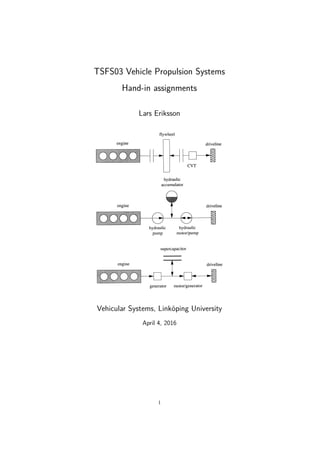
  • 26. 4.1.2 Design of new vehicle Choose a short term storage concept. You may for example choose one of the concepts from Figure 5.2 in [1]. However, you are free to connect any components you wish as long as it’s physically feasible and provided that you add the components masses to the vehicle mass. Write down the equations for all the components of the modeled vehicle. Then chose component sizes, gear ratios and other quantities. Plot finally the efficiency maps as well as limiting factors where applicable and ensure that 1. All operating points will be within the limits for the used components. 2. The components will be operating close to the maximum efficiency when working together. 3. The short term storage system[s] are large enough. If you are uncertain of how to implement your concept in QSS you may look at the QSS built-in examples, especially qss example shv. Also remember that the Matlab/Simulink blocks Scope and To Workspace are your friends. 4.1.3 Design of control strategy A control strategy is an algorithm that decides where to take the energy that is needed by the vehicle-drivecycle pair and how to utilize the short term storage. The control strategy should be designed so that the vehicle can perform the whole drive cycle without running into torque/speed limits and so that the combustion engine as well as the other components are operated in an efficient way. 4.1.4 Evaluation of new Vehicle and control strategy Show how your vehicle/control-strategy works together. Use efficiency plots that show what operating points your components are operating in. Have you chosen the right gear ratios and sizes for your vehicle? Make a parameter study to see how sensitive your fuel consumption is to the model parameters for your short term storage components as well as your control strategy. Here it is important to not favor parameter choices that drains the short term storage system. Also make believable that your fuel consumption is accurate. That is, ex- plain where your design saves the most fuel and how this affects the total fuel consumption. 4.2 Available models and assumptions First is a list of the available components you are allowed to add as well as common model assumptions and then a detailed walk through of some of the components. • Flywheels • Hydraulic Accumulators • Supercapacitors 26
  • 27. as well as the following glue components • Gearboxes • Electric motors • Electric generators • Continously variable transmissions • Hydraulic pumps/motors • Torque couplers and planetary gear sets • Power electronics All short term storage devices should have the same, or higher, charge status after the driving cycle as before, otherwise this has to be accounted for in a realistic way. 4.2.1 Short term storage systems The equations for the short term storage systems are specified in the course literature unless available here as a reference. Parameters are to be chosen within reasonable limitations. Investigate how different parameters (e.g. the speed of the flywheel, charge of the hydraulic accumulator or supercapacitor, and power) affect the efficiency of the component(s) used. This can e.g. be done using the Peukert or Ragone tests for the supercapacitor and hydraulic accumulator. Flywheel Assume that you are able to make flywheels using a material with ρ = 8000 [kg/m3 ] and are able to choose b, d and q freely within reasonable limits. Also assume that manufacturing limitations gives you the flywheel parameters in Table 4.1. Assume that the total weight of the flywheel and bearings is 5% more than the flywheel mass. Parameter Description Value ρ Flywheel density 8000 [kg/m3 ] ρa Ambient air density 1.29 [kg/m3 ] ηa Dynamic air viscosity 1.72 ·10−5 [Pa s] b Width By choice d Diameter By choice q Inner/Outer diameter ratio q ∈ [0, 1] dw/d Shaft/Wheel ratio 0.08 [-] µ Friction coefficient 1.5 · 10−3 [-] k Unbalance factor 4 [-] ωmax Maximum speed 30 000 [rpm] mtot Total mass 1.05 · mf Table 4.1: Flywheel parameters from the flywheel manufacturer. 27
  • 28. Hydraulic accumulator Assume that the hydraulic accumulator may be described by a thermodynamic model together with the parameters in Table 4.2. Also assume that the total weight of the accumulator and its components are described by the equations for a spheric accumulator and that the weight of the metal shell is negligible. The weight of the oil should be at maximum charge. Note the importance of choosing the capacities so that the maximum pressure is never exceeded. It is Parameter Description Value Vg,max Maximum gas capacity By choice Vg,min Minimum gas capacity By choice fc Fluid capacity By choice ρoil Hydraulic oil density 900 [kg/m3 ] Tw Wall temperature 320 [K] Rg Gas constant 520 [J/kgK] pmax Maximum pressure [400-800] [bar] pinit Pre charge pressure 125 [bar] Tinit Pre charge temperature 320 [K] h Heat transfer coefficient 100 [W/Km2 ] Table 4.2: Hydraulic accumulator parameters from the manufacturer. advantageous to look at the implementation details for the Supercapacitor from the QSS library during the implementation. Use the volume fraction as state of charge. Supercapacitor Use the equations from the equivalent circuit paragraph in the literature and the parameters in Table 4.3 below. You are free to use as many as necessary. Parameter Description Value CSC Capacity per supercap 8 [F] RSC Internal resistance 0.72 [Ohm] Vmax,SC Maximum voltage of supercap 225 [V] Pmax,SC Maximum power drain of supercap 175 [kW] ESC Specific energy of supercap 2 [Wh/kg] Table 4.3: Model parameters and assumptions supercapacitor 4.2.2 Glue components The equations for the glue components are specified in the course literature un- less available here as a reference. Parameters are to be chosen within reasonable limitations unless specified. 28
  • 29. Gearbox The gearbox equations are Pout = ηGB · Pin − P0 ωin = ωout · ix where P0 is the friction losses and is direction dependent. (See for example the gearbox implementation in the QSS library.) The model parameters are listed in Table 4.4. Parameter Description Value ηGB Gearbox efficiency 0.98 [-] P0 Constant term in losses 50 [W] m Gearbox mass 10 [kg/gear] Table 4.4: Model parameters and assumptions for a manual gearbox Continously variable transmission Assume that the CVT can be described as a normal gearbox but with a lower efficiency and higher idling losses. Parameters are listed in Table 4.5. Parameter Description Value ηGB Gearbox efficiency 0.93 [-] P0 Constant term in losses 400 [W] m Gearbox mass 10 [kg] Table 4.5: Model parameters and assumptions for a CVT gearbox In a CVT there is an upper limit in how fast the gear ratio can be changed, as well as a torque limit. However, these limitation are neglected in this task. Hydraulic pump/motor Use the Willans approach with the parameters in Table 4.6 below. Parameter Description Value P0 Idling losses 300 [W] e Efficiency 0.8 [-] m Hydraulic pump mass 10 [kg] Table 4.6: Model parameters and assumptions for hydraulic pump/motor Torque coupler and planetary gear set Assume that your torque couplers and or planetary gear sets are ideal without losses. Power electronics Neglect any power losses. 29
  • 30. 4.2.3 Energy converters Electric motor Assume that the electric motor is of the type from the QSS library. To help get you started the command mkPlots.m is available for download. The code shows how to plot engine performance maps and gives you an idea of how the efficiency of the electric motor in the QSS library is modeled. In Figure 4.1 the efficiency map for the electric motor has been plotted together with the torque limit. Assume that your engine is scalable using the scale parameter and the weight of the component and the power electronics is 1.5 kg/kW. 0.7 0.70.7 0.7 0.7 0.7 0.7 0.7 0.7 0.7 0.75 0.75 0.75 0.75 0.75 0.75 0.75 0.75 0.75 0.75 0.75 0.8 0.8 0.8 0.8 0.8 0.8 0.8 0.8 0.8 0.8 0.8 0.8 0.8 0.8 0.825 0.825 0.825 0.825 0.825 0.825 0.825 0.825 0.825 0.825 0.825 0.825 0.825 0.825 0.85 0.85 0.85 0.85 0.85 0.85 0.85 0.85 0.85 0.85 ωEM [rad/s] T EM [Nm] Electric Motor map 0 100 200 300 400 500 600 −60 −40 −20 0 20 40 60 Figure 4.1: Performace map of electric motor from the QSS library Electric generator As with the electric motor assume that the electric generator is of the type from the QSS library. The command mkPlots.m is available for download to help you get started with plotting engine performance maps and get an idea of how the efficiency of the electric generator in the QSS library is implemented. In Figure 4.2 the efficiency map for the electric motor has been plotted together with the torque limit. Assume that the generator is scalable using the scale parameter and the weight of the component and power electronics is 1.5 kg/kW. Combustion engine A map based engine model is used in this task. The fuel consumption is tabu- lated and is estimated given the torque and speed of the engine. The parameters to be used are given in OrdinaryVehicle.mdl. If you change the size of the engine, approximate the change in weight to 1.2 kg/kW. 30
  • 31. 0.7 0.7 0.7 0.7 0.7 0.7 0.7 0.75 0.75 0.75 0.75 0.75 0.75 0.75 0.75 0.75 0.8 0.8 0.8 0.8 0.8 0.8 0.8 0.83 0.83 0.83 0.83 0.83 0.85 0.85 ω EG [rad/s] TEG [Nm] Electric Generator map 0 100 200 300 400 500 600 10 20 30 40 50 60 70 Figure 4.2: Performace map of electric generator from the QSS library Combustion Engine map and usage (ordinary) ω CE [rad/s] T CE [Nm] 0.1 0.2 0.275 0.3 0.325 100 200 300 400 500 600 700 800 0 20 40 60 80 100 120 140 160 180 200 Figure 4.3: Performace map of combustion engine using the map based engine model 31
  • 32. Hand-In 5 Fuel Cell and Supervisory Control This hand-in is not mandatory, but is an extra task that gives up to 14 points. Purpose In this hand-in you are supposed to implement a fuel cell vehicle in Simulink using forward modeling. The purpose is twofold: • get knowledge about how a fuel cell works and evaluate efficiencies and fuel consumption of a fuel cell vehicle. • get familiar with forward modeling. Examination requirement • The vehicle should fulfill the specifications given in section 5.1.1. • Calculate the fuel consumption using hydrogen as fuel. The fuel con- sumption is preferably presented in equivalent gasoline consumption per 100 km. Use NEDC. • Calculate the fuel consumption if methanol is used as fuel instead of hy- drogen, (use information in section 5.2.1). Compare this result to a con- ventional vehicle equipped with an SI engine. Make the comparison in terms of both the energy consumption and CO2 emissions. Hint: To calculate the CO2 emissions, assume stoichiometric mixture. Use the results from hand-in 1 for the conventional vehicle. • Calculate the average efficiency of the fuel cell, electric machine and the buffer. 32
  • 33. 5.1 Assignment specification The assignment is to be solved using Simulink and a given model skeleton that can be downloaded from the course homepage. Chapter 6 in the Vehicle Propul- sion System book [1] covers fuel cells. It might also be helpful to study the model implemented in QSS. The final report must at least contain the following: • Description and discussion of the design, including values of important parameters of your model. • Description and discussion of your chosen control strategy. • Plots showing the efficiency and operating points of your components. The report should be self explanatory and all the components included in the model must be documented. All assumptions should be discussed and the con- trol strategy should be well described, discussed, and motivated. You should also evaluate and provide support for the credibility of your fuel consumption estimate. Furthermore, you should explain where your design saves the most fuel and how this affects the total fuel consumption. 5.1.1 Vehicle demands To be able to compare the conventional vehicle to the vehicle developed in this assignment, the vehicle should manage to • accelerate from stand still to 100 km/h in 15 s, • have a sustained top speed of at least 160 km/h, and • have high overall efficiency on the NEDC. Vehicle and component parameters, such as the specific weights, are given in section 5.3. 5.1.2 Design of new vehicle Write down the equations for all the components of the modeled vehicle. Then choose component sizes and other quantities. Make sure the vehicle fulfills the requirements in section 5.1.1. Finally plot the efficiencies (for the fuel cell, this could be efficiency against power), as well as limiting factors where applicable. Ensure that 1. all operating points will be within the limits for the used components, 2. the components will be operating close to the maximum efficiency when working together, and 3. the short term storage system[s] are large enough. 5.1.3 Design of control strategy A control strategy with the same demands as described in section 4.1.3 is to be implemented. 33
  • 34. 5.2 Available models and assumptions There are some models included in the skeleton that you can use. You are of course free to develop and add new models of the components. Skeletons for the controller and fuel cell are included in the given skeleton, which you are to add functionality to. Observe that the vehicle model is sensitive for naming of the signals, since buses are used. The parameters of the components are to be chosen in order to fulfill the requirements in section 5.1.1. You are free to choose any configuration of the vehicle you want to, as long as it is physically possible to construct. There is one concept of a fuel cell vehicle chosen in the given skeleton that you can use. 5.2.1 Fuel You are supposed to implement a model of a vehicle that uses hydrogen as fuel, i.e. there is no reformer in the vehicle. This should result in a relatively high overall efficiency of the vehicle. The disadvantages associated with this technol- ogy are for example that hydrogen storage is problematic, new infrastructure is needed, and that transportation of hydrogen is costly. An alternative is to use methanol as fuel and use a reformer on-board that produces hydrogen. Assume that the reformer has a mean efficiency of 55 %, and that the lower heating value of methanol is 19.8 MJ/kg. 5.3 Vehicle Data In this section some data to be used in the modeling of the fuel cell vehicle is given. For the data not presented in this section, use the parameters for the sports car in Hand-in 1. 5.3.1 Fuel cell The fuel cell has slower dynamics than for example an ICE. Therefore it is not adequate to assume that the requested power from the fuel cell is delivered instantaneously, if there is a change in the power demanded. In this task this is modeled using a first order low pass filter with a time constant of 5 seconds. Data needed for one cell in the stack is given in Table 5.1. 5.3.2 Super capacitor A buffer consists of several cells connected in series and in some cases paral- lel. You are free to design the buffer as long as you use realistic parameters. The following data for a cell in the super capacitor is just an example of the magnitude of the parameters. The capacitance is 3 F, voltage 2.5 V and inner resistance 2 mΩ. The inner resistance is a relative large value. This is to model the losses due to leakage currents in the capacitor since that is not a part of the given model. If you wish to use other parameters http://www.maxwell.com is a good place to start looking. 34
  • 35. Parameter Description Value Vth Theoretical voltage at Ifc = 0 1.3 [V] V0 Voltage at Ifc = 0 in linear approx. 0.88 [V] Afc Fuel cell area 0.3 [m2 ] ˜R Normalized resistance 0.00008 [Ω m2 ] λ Air/fuel ratio 1.5 [-] Mair Molar mass of air 29.0 [kg/kmol] qlhv,hydrogen Lower heating value of hydrogen 285.9 MJ/kmol ηem Efficiency of em driving compressor 0.75 [-] ηcomp Efficiency of compressor 0.70 [-] Π Compression ratio 1.3 [-] Pidle Minimum power from fuel cell stack 1000 [W] Tamb Ambient temperature 298 [K] Table 5.1: Model parameters for one fuel cell. Use the data to model a stack. 5.3.3 Electric machine You are free to model the electric machine in any way that you prefer, as long as it is realistic and you describe the model. If you use the model given in the skeleton, the data presented in table 5.2 might be useful. Parameter Description Value R Inner resistance 0.35 [Ω] J Inertia 0.2 [kgm2 ] ka Torque constant 0.50 [Nm/A] ki voltage/speed constant 0.51 [Vs/rad] Table 5.2: Model parameters for the electric machine using the model electric- motor quasistatic2 std. In this model the power electronics is included converting the voltage of the buffer to the requested voltage of the electric machine. 5.3.4 Vehicle mass The mass of the vehicle depends on the design of the components used. To be able to estimate the mass of the vehicle, the following information is to be used: • the vehicle body weight 900 kg including a pay-load of 100 kg, • the fuel cell weight 2 kg/kW where the power is the peak power of the fuel cell. • The electric system including e.g. electric machine and power electronics has a mass of 1.5 kg/kW and • the specific power of the super capacitor is 10 kW/kg and the specific energy 4 Wh/kg. In this task the weight of the super capacitor is assumed to be the maximum value of the two ways of estimating the weight. 35
  • 36. You are free to use a battery instead of the super capacitor. If you do so you have to find information about the weight of the battery used in the modeled vehicle. 36
  • 37. Bibliography [1] Lino Guzzella and Antoni Sciarretta. Vehicle Propulsion Systems – Intro- duction to Modeling and Optimization. Springer Verlag, 3 edition, 2013. 37