1. Motivation: Association Rule Mining
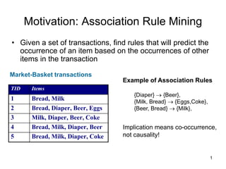
• Given a set of transactions, find rules that will predict the
occurrence of an item based on the occurrences of other
items in the transaction
Market-Basket transactions
TID Items
1 Bread, Milk
2 Bread, Diaper, Beer, Eggs
3 Milk, Diaper, Beer, Coke
4 Bread, Milk, Diaper, Beer
5 Bread, Milk, Diaper, Coke
Example of Association Rules
{Diaper} {Beer},
{Milk, Bread} {Eggs,Coke},
{Beer, Bread} {Milk},
Implication means co-occurrence,
not causality!
1
2. Applications: Association Rule Mining
• * Maintenance Agreement
– What the store should do to boost Maintenance
Agreement sales
• Home Electronics *
– What other products should the store stocks up?
• Attached mailing in direct marketing
• Detecting “ping-ponging” of patients
• Marketing and Sales Promotion
• Supermarket shelf management
2
3. Definition: Frequent Itemset
• Itemset
– A collection of one or more items
• Example: {Milk, Bread, Diaper}
– k-itemset
• An itemset that contains k items
• Support count ()
– Frequency of occurrence of an itemset
– E.g. ({Milk, Bread,Diaper}) = 2
• Support
– Fraction of transactions that contain an
itemset
– E.g. s({Milk, Bread, Diaper}) = 2/5
• Frequent Itemset
– An itemset whose support is greater
than or equal to a minsup threshold
TID Items
1 Bread, Milk
2 Bread, Diaper, Beer, Eggs
3 Milk, Diaper, Beer, Coke
4 Bread, Milk, Diaper, Beer
5 Bread, Milk, Diaper, Coke
3
4. Definition: Association Rule
Example:
Beer
}
Diaper
,
Milk
{
4
.
0
5
2
|
T
|
)
Beer
Diaper,
,
Milk
(
s
67
.
0
3
2
)
Diaper
,
Milk
(
)
Beer
Diaper,
Milk,
(
c
• Association Rule
– An implication expression of the form
X Y, where X and Y are itemsets
– Example:
{Milk, Diaper} {Beer}
• Rule Evaluation Metrics
– Support (s)
• Fraction of transactions that contain
both X and Y
– Confidence (c)
• Measures how often items in Y
appear in transactions that
contain X
TID Items
1 Bread, Milk
2 Bread, Diaper, Beer, Eggs
3 Milk, Diaper, Beer, Coke
4 Bread, Milk, Diaper, Beer
5 Bread, Milk, Diaper, Coke
4
5. Association Rule Mining Task
• Given a set of transactions T, the goal of
association rule mining is to find all rules having
– support ≥ minsup threshold
– confidence ≥ minconf threshold
• Brute-force approach:
– List all possible association rules
– Compute the support and confidence for each rule
– Prune rules that fail the minsup and minconf
thresholds
Computationally prohibitive!
5
6. Computational Complexity
• Given d unique items:
– Total number of itemsets = 2d
– Total number of possible association rules:
1
2
3 1
1
1 1
d
d
d
k
k
d
j
j
k
d
k
d
R
If d=6, R = 602 rules
6
7. Mining Association Rules: Decoupling
Example of Rules:
{Milk,Diaper} {Beer} (s=0.4, c=0.67)
{Milk,Beer} {Diaper} (s=0.4, c=1.0)
{Diaper,Beer} {Milk} (s=0.4, c=0.67)
{Beer} {Milk,Diaper} (s=0.4, c=0.67)
{Diaper} {Milk,Beer} (s=0.4, c=0.5)
{Milk} {Diaper,Beer} (s=0.4, c=0.5)
TID Items
1 Bread, Milk
2 Bread, Diaper, Beer, Eggs
3 Milk, Diaper, Beer, Coke
4 Bread, Milk, Diaper, Beer
5 Bread, Milk, Diaper, Coke
Observations:
• All the above rules are binary partitions of the same itemset:
{Milk, Diaper, Beer}
• Rules originating from the same itemset have identical support but
can have different confidence
• Thus, we may decouple the support and confidence requirements 7
8. Mining Association Rules
• Two-step approach:
1. Frequent Itemset Generation
– Generate all itemsets whose support minsup
2. Rule Generation
– Generate high confidence rules from each frequent itemset,
where each rule is a binary partitioning of a frequent itemset
• Frequent itemset generation is still
computationally expensive
8
9. Frequent Itemset Generation
• Brute-force approach:
– Each itemset in the lattice is a candidate frequent itemset
– Count the support of each candidate by scanning the
database
– Match each transaction against every candidate
– Complexity ~ O(NMw) => Expensive since M = 2d !!!
TID Items
1 Bread, Milk
2 Bread, Diaper, Beer, Eggs
3 Milk, Diaper, Beer, Coke
4 Bread, Milk, Diaper, Beer
5 Bread, Milk, Diaper, Coke
N
Transactions List of
Candidates
M
w
9
10. Frequent Itemset Generation Strategies
• Reduce the number of candidates (M)
– Complete search: M=2d
– Use pruning techniques to reduce M
• Reduce the number of transactions (N)
– Reduce size of N as the size of itemset increases
– Use a subsample of N transactions
• Reduce the number of comparisons (NM)
– Use efficient data structures to store the candidates or
transactions
– No need to match every candidate against every
transaction
10
11. Reducing Number of Candidates: Apriori
• Apriori principle:
– If an itemset is frequent, then all of its subsets must also
be frequent
• Apriori principle holds due to the following property
of the support measure:
– Support of an itemset never exceeds the support of its
subsets
– This is known as the anti-monotone property of support
)
(
)
(
)
(
:
, Y
s
X
s
Y
X
Y
X
11
12. Found to be
Infrequent
null
AB AC AD AE BC BD BE CD CE DE
A B C D E
ABC ABD ABE ACD ACE ADE BCD BCE BDE CDE
ABCD ABCE ABDE ACDE BCDE
ABCDE
Illustrating Apriori Principle
null
AB AC AD AE BC BD BE CD CE DE
A B C D E
ABC ABD ABE ACD ACE ADE BCD BCE BDE CDE
ABCD ABCE ABDE ACDE BCDE
ABCDE
Pruned
supersets 12
13. Illustrating Apriori Principle
Item Count
Bread 4
Coke 2
Milk 4
Beer 3
Diaper 4
Eggs 1
Itemset Count
{Bread,Milk} 3
{Bread,Beer} 2
{Bread,Diaper} 3
{Milk,Beer} 2
{Milk,Diaper} 3
{Beer,Diaper} 3
Itemset Count
{Bread,Milk,Diaper} 3
Items (1-itemsets)
Pairs (2-itemsets)
(No need to generate
candidates involving Coke
or Eggs)
Triplets (3-itemsets)
Minimum Support = 3
If every subset is considered,
6C1 + 6C2 + 6C3 = 41
With support-based pruning,
6 + 6 + 1 = 13
13
14. Apriori Algorithm
• Method:
– Let k=1
– Generate frequent itemsets of length 1
– Repeat until no new frequent itemsets are identified
• Generate length (k+1) candidate itemsets from length k
frequent itemsets
• Prune candidate itemsets containing subsets of length k that
are infrequent
• Count the support of each candidate by scanning the DB
• Eliminate candidates that are infrequent, leaving only those
that are frequent
14
15. Apriori: Reducing Number of Comparisons
• Candidate counting:
– Scan the database of transactions to determine the support of
each candidate itemset
– To reduce the number of comparisons, store the candidates in a
hash structure
• Instead of matching each transaction against every candidate,
match it against candidates contained in the hashed buckets
TID Items
1 Bread, Milk
2 Bread, Diaper, Beer, Eggs
3 Milk, Diaper, Beer, Coke
4 Bread, Milk, Diaper, Beer
5 Bread, Milk, Diaper, Coke
N
Transactions Hash Structure
k
Buckets 15
18. 18
Apriori: A Candidate Generation-and-Test
Approach
• Apriori pruning principle: If there is any itemset which is
infrequent, its superset should not be generated/tested!
(Agrawal & Srikant @VLDB’94, Mannila, et al. @ KDD’ 94)
• Method:
– Initially, scan DB once to get frequent 1-itemset
– Generate length (k+1) candidate itemsets from length k
frequent itemsets
– Test the candidates against DB
– Terminate when no frequent or candidate set can be
generated
20. 20
The Apriori Algorithm
• Pseudo-code:
Ck: Candidate itemset of size k
Lk : frequent itemset of size k
L1 = {frequent items};
for (k = 1; Lk !=; k++) do begin
Ck+1 = candidates generated from Lk;
for each transaction t in database do
increment the count of all candidates in Ck+1
that are contained in t
Lk+1 = candidates in Ck+1 with min_support
end
return k Lk;
21. 21
Important Details of Apriori
• How to generate candidates?
– Step 1: self-joining Lk
– Step 2: pruning
• How to count supports of candidates?
• Example of Candidate-generation
– L3={abc, abd, acd, ace, bcd}
– Self-joining: L3*L3
• abcd from abc and abd
• acde from acd and ace
– Pruning:
• acde is removed because ade is not in L3
– C4={abcd}
22. 22
How to Generate Candidates?
• Suppose the items in Lk-1 are listed in an order
• Step 1: self-joining Lk-1
insert into Ck
select p.item1, p.item2, …, p.itemk-1, q.itemk-1
from Lk-1 p, Lk-1 q
where p.item1=q.item1, …, p.itemk-2=q.itemk-2, p.itemk-1 < q.itemk-
1
• Step 2: pruning
forall itemsets c in Ck do
forall (k-1)-subsets s of c do
if (s is not in Lk-1) then delete c from Ck
23. 23
How to Count Supports of Candidates?
• Why counting supports of candidates a problem?
– The total number of candidates can be very huge
– One transaction may contain many candidates
• Method:
– Candidate itemsets are stored in a hash-tree
– Leaf node of hash-tree contains a list of itemsets and
counts
– Interior node contains a hash table
– Subset function: finds all the candidates contained in
a transaction
25. 25
Challenges of Frequent Pattern Mining
• Challenges
– Multiple scans of transaction database
– Huge number of candidates
– Tedious workload of support counting for candidates
• Improving Apriori: general ideas
– Reduce passes of transaction database scans
– Shrink number of candidates
– Facilitate support counting of candidates
26. 26
Partition: Scan Database Only Twice
• Any itemset that is potentially frequent in DB must be
frequent in at least one of the partitions of DB
– Scan 1: partition database and find local frequent
patterns
– Scan 2: consolidate global frequent patterns
• A. Savasere, E. Omiecinski, and S. Navathe. An efficient
algorithm for mining association in large databases. In
VLDB’95
27. 27
DHP: Reduce the Number of Candidates
• A k-itemset whose corresponding hashing bucket count is
below the threshold cannot be frequent
– Candidates: a, b, c, d, e
– Hash entries: {ab, ad, ae} {bd, be, de} …
– Frequent 1-itemset: a, b, d, e
– ab is not a candidate 2-itemset if the sum of count of
{ab, ad, ae} is below support threshold
• J. Park, M. Chen, and P. Yu. An effective hash-based
algorithm for mining association rules. In SIGMOD’95
29. • Traversal of Itemset Lattice
– Breadth-first vs Depth-first
(a) Breadth first (b) Depth first
Apriori: Alternative Search Methods
29
30. Bottlenecks of Apriori
• Candidate generation can result in huge
candidate sets:
– 104 frequent 1-itemset will generate 107 candidate 2-
itemsets
– To discover a frequent pattern of size 100, e.g., {a1,
a2, …, a100}, one needs to generate 2100 ~ 1030
candidates.
• Multiple scans of database:
– Needs (n +1 ) scans, n is the length of the longest
pattern
30
31. ECLAT: Another Method for Frequent Itemset
Generation
• ECLAT: for each item, store a list of transaction
ids (tids); vertical data layout
TID Items
1 A,B,E
2 B,C,D
3 C,E
4 A,C,D
5 A,B,C,D
6 A,E
7 A,B
8 A,B,C
9 A,C,D
10 B
Horizontal
Data Layout
A B C D E
1 1 2 2 1
4 2 3 4 3
5 5 4 5 6
6 7 8 9
7 8 9
8 10
9
Vertical Data Layout
TID-list 31
32. ECLAT: Another Method for Frequent Itemset
Generation
• Determine support of any k-itemset by intersecting tid-
lists of two of its (k-1) subsets.
• 3 traversal approaches:
– top-down, bottom-up and hybrid
• Advantage: very fast support counting
• Disadvantage: intermediate tid-lists may become too
large for memory
A
1
4
5
6
7
8
9
B
1
2
5
7
8
10
AB
1
5
7
8
32
33. FP-growth: Another Method for Frequent
Itemset Generation
• Use a compressed representation of the
database using an FP-tree
• Once an FP-tree has been constructed, it uses a
recursive divide-and-conquer approach to mine
the frequent itemsets
33
38. FP-growth
Conditional pattern base
for D within conditional
base for E:
P = {(A:1,C:1,D:1),
(A:1,D:1)}
Count for D is 2: {D,E} is
frequent itemset
Recursively apply FP-
growth on P
Conditional tree for D
within conditional tree
for E:
null
A:2
C:1
D:1
D:1
38
39. FP-growth
Conditional pattern base
for C within D within E:
P = {(A:1,C:1)}
Count for C is 1: {C,D,E}
is NOT frequent itemset
Conditional tree for C
within D within E:
null
A:1
C:1
39
40. FP-growth
Count for A is 2: {A,D,E}
is frequent itemset
Next step:
Construct conditional tree
C within conditional tree
E
Continue until exploring
conditional tree for A
(which has only node A)
Conditional tree for A
within D within E:
null
A:2
40
41. Benefits of the FP-tree Structure
• Performance study shows
– FP-growth is an order of
magnitude faster than
Apriori, and is also faster
than tree-projection
• Reasoning
– No candidate generation,
no candidate test
– Use compact data structure
– Eliminate repeated
database scan
– Basic operation is counting
and FP-tree building
0
10
20
30
40
50
60
70
80
90
100
0 0.5 1 1.5 2 2.5 3
Support threshold(%)
Run
time(sec.)
D1 FP-grow th runtime
D1 Apriori runtime
41
42. Complexity of Association Mining
• Choice of minimum support threshold
– lowering support threshold results in more frequent itemsets
– this may increase number of candidates and max length of
frequent itemsets
• Dimensionality (number of items) of the data set
– more space is needed to store support count of each item
– if number of frequent items also increases, both computation and
I/O costs may also increase
• Size of database
– since Apriori makes multiple passes, run time of algorithm may
increase with number of transactions
• Average transaction width
– transaction width increases with denser data sets
– This may increase max length of frequent itemsets and traversals
of hash tree (number of subsets in a transaction increases with its
width)
42
43. Maximal Frequent Itemset
null
AB AC AD AE BC BD BE CD CE DE
A B C D E
ABC ABD ABE ACD ACE ADE BCD BCE BDE CDE
ABCD ABCE ABDE ACDE BCDE
ABCD
E
Border
Infrequent
Itemsets
Maximal
Itemsets
An itemset is maximal frequent if none of its immediate supersets
is frequent
43
44. Closed Itemset
• Problem with maximal frequent itemsets:
– Support of their subsets is not known – additional DB scans are
needed
• An itemset is closed if none of its immediate supersets
has the same support as the itemset
TID Items
1 {A,B}
2 {B,C,D}
3 {A,B,C,D}
4 {A,B,D}
5 {A,B,C,D}
Itemset Support
{A} 4
{B} 5
{C} 3
{D} 4
{A,B} 4
{A,C} 2
{A,D} 3
{B,C} 3
{B,D} 4
{C,D} 3
Itemset Support
{A,B,C} 2
{A,B,D} 3
{A,C,D} 2
{B,C,D} 2
{A,B,C,D} 2
44
45. Maximal vs Closed Frequent Itemsets
null
AB AC AD AE BC BD BE CD CE DE
A B C D E
ABC ABD ABE ACD ACE ADE BCD BCE BDE CDE
ABCD ABCE ABDE ACDE BCDE
ABCDE
124 123 1234 245 345
12 124 24 4 123 2 3 24 34 45
12 2 24 4 4 2 3 4
2 4
Minimum support = 2
# Closed = 9
# Maximal = 4
Closed and
maximal
Closed but
not maximal
TID Items
1 ABC
2 ABCD
3 BCE
4 ACDE
5 DE
45
47. Rule Generation
• Given a frequent itemset L, find all non-empty
subsets f L such that f L – f satisfies the
minimum confidence requirement
– If {A,B,C,D} is a frequent itemset, candidate rules:
ABC D, ABD C, ACD B, BCD A,
A BCD, B ACD, C ABD, D ABC
AB CD, AC BD, AD BC, BC AD,
BD AC, CD AB,
• If |L| = k, then there are 2k – 2 candidate
association rules (ignoring L and L)
47
48. Rule Generation
• How to efficiently generate rules from frequent
itemsets?
– In general, confidence does not have an anti-
monotone property
c(ABC D) can be larger or smaller than c(AB D)
– But confidence of rules generated from the same
itemset has an anti-monotone property
– e.g., L = {A,B,C,D}:
c(ABC D) c(AB CD) c(A BCD)
• Confidence is anti-monotone w.r.t. number of items on the
RHS of the rule 48