basic commands,syntax

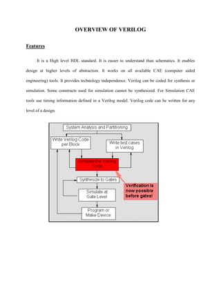
1. OVERVIEW OF VERILOG
Features
It is a High level HDL standard. It is easier to understand than schematics. It enables
design at higher levels of abstraction. It works on all available CAE (computer aided
engineering) tools. It provides technology independence. Verilog can be coded for synthesis or
simulation. Some constructs used for simulation cannot be synthesized. For Simulation CAE
tools use timing information defined in a Verilog model. Verilog code can be written for any
level of a design.

2. begin...end Block Statements
Using block statements is a way of syntactically grouping several statements into a single
statement. In Verilog , sequential blocks are delimited by the keywords begin and end. These
begin...end pairs are commonly used in conjunction with if, case, and for statements to group
several statements. Functions and always blocks that contain more than one statement require a
begin...end pair to group the statements. Verilog also provides a construct called a named block.
Block Statement With a Named Block
begin : block_name
reg local_variable_1;
integer local_variable_2;
parameter local_variable_3;
... statements ...
end
if...else Statements
The if ... else statements execute a block of statements according to the value of one or more
expressions.
The syntax of if...else statements is
if ( e xpr )
begin
... statements ...

3. end
else
begin... statements ..
end
The if statement consists of the keyword if followed by an expression in parenthesis. If
statement is followed by a statement or block of statements enclosed by begin and end.
case Statements
The case statement is similar in function to the if...else conditional statement. The case
statement allows a multi path branch in logic that is based on the value of an expression. One
way to describe a multi cycle circuit is with a case statement. Another way is with multiple @
(clock edge) statements, which are discussed in the subsequent sections on loops.
The syntax for a case statement is
case ( expr )
case_item1: begin
... statements ...
end
case_item2: begin
... statements ...
end
default: begin
... statements ...

4. end
endcase
The case statement consists of the keyword case, followed by an expression in
parentheses, followed by one or more case items (and associated statements to be executed),
followed by the keyword endcase. A case item consists of an expression (usually a simple
constant) or a list of expressions separated by commas, followed by a colon (:). The expression
following the case keyword is compared with each
case item expression, one by one. When the expressions are equal, the condition evaluates to
true. Multiple expressions separated by commas can be used in each case item. When multiple
expressions are used, the condition is said to be true if any of the expressions in the case item
match the expression following the case keyword.
CasexStatements
The casex statement allows a multi path branch in logic, according to the value of an
expression, just as the case statement does. The differences between the case statement and the
casex statement are the keyword and the processing of the expressions.
The syntax for a casex statement is
casex ( expr )
case_item1: begin
... statements ...
end
case_item2: begin
... statements ...

5. end
default: begin
... statements ...
end
endcase
casex Statements
The casex statement allows a multi path branch in logic, according to the value of an
expression, just as the case statement does. The differences between the case statement and the
casex statement are the keyword and the processing of the expressions.
The syntax for a casex statement is
casex ( expr )
case_item1: begin
... statements ...
end
case_item2: begin
... statements ...
End
default: begin
... statements ...
end
endcase

6. Programming Statements …case
Syntax:
case (net_or_register_or_literal)
case_match1: statement or statement_group
case_match2: ……………..
case_match3: statement or statement_group
default: statement or statement_group
endcase
Forever Statement
This loop executes continuously and never completes that is an infinite loop that
continuously executes the statement or statement group. Infinite loops in Verilog use the
keyword forever. You must break up an infinite loop with an @ (posedge clock) or @ (negedge
clock).
Procedural Assignment
Procedural assignments are assignment statements used inside a function, except that the
left side of a procedural assignment can contain only reg, variables and integers. Assignment
statements set the value of the left side to the current value of the right side. The right side of
the assignment can contain any arbitrary expression of the data types. The value placed on a
variable will remain unchanged until another procedural assignment updates the variable with a
different value.

7. Blocking and Non-Blocking statements are procedural assignments used to update/assign a
signal value. Assignments can be scalar or vector. Two types of procedural assignment can be
made Blocking: Sequential Operation, Operator = or Non-Blocking: Concurrent Operation,
Operator <=
Blocking:
Statement1 Statement2 Statement3
Non Blocking:
Statement1
|
Statement 2
|
Statement 3
Procedural Assignments (Blocking)
register_data_type = expression;
Blocking assignment statement execute in the order they are specified in sequential block.
Expression is evaluated and assigned when the statement is encountered. In a begin--end
sequential statement group, execution of the next statement is blocked until the assignment is
complete. In the sequence begin m=n; n=m; end, the 1st assignment changes m before the 2nd
assignment evaluates m.
Procedural Assignments (Non-Blocking)
register_data_type <= expression;

8. Expression is evaluated when the statement is encountered, and assignment is
postponed until the end of the time-step. In begin--end sequential statement group, execution of
the next statement is not blocked; and may be evaluated before the assignment is complete. In
the sequence begin m<=n; n<=m; end, both assignments will be evaluated before m or n
changes.
Repeat Statement
Repeat (number) statement or statement group. A loop that executes the statement or
statement group a set number of times. Number may be an integer, a variable, or an expression (a
variable or expression is only evaluated when the loop is first entered).
While Statement
While (expression) statement or statement_group. The while loop executes a statement
until the controlling expression evaluates to false. A while loop creates a conditional branch that
must be broken by one of the following statements to prevent combinational feedback.
Unsupported & Supported while Loop
Unsupported while Loop
always
while (x < y)
x = x + z;
Supported while Loop
always

9. begin @ (posedge clock)
while (x < y)
begin
@ (posedge clock);
x = x + z;
end
end;
For Statement
For (initial_assignment; expression; step_assignment) statement or statement_group. It
executes initial_assignment once when the loop starts. Executes the statement or statement
group as long as the expression evaluates as true. Executes the step_assignment at the end of
each pass through the loop.
Example for 3 to 8 Encoder.
module enc3to8 (out,in);
input [7:0] in;
output [2:0] out;
reg [7:0] out;
integer i;
always @ (in)
begin

10. out = 0;
for (i=0; i < 8;i=i+1)
if (in[i])
out = i;
end
endmodule
Test Benches in Verilog.
Test benches prove that a design is correct. How do you create a simple testbench in
Verilog?
Let’s take the MUX_2 example module and create a testbench for it. We can create a template
for the testbench code.
module MUX2TEST;
// No ports!
...
initial
// Stimulus
... MUX2 M (SEL, A, B, F); initial

11. // Analysis
...
endmodule
In this code, the stimulus and response capture are going to be coded using a pair of initial
blocks. An initial block can contain sequential statements that can be used to describe the
behaviour of signals in a test bench. In the Stimulus initial block, we need to generate waveform
on the A, B and SEL inputs.
Structural data type
Wire:
A wire data type in a Verilog description represents the physical wires in a circuit. A wire
connects gate-level instantiations and module instantiations. The Verilog language allows you to
read a value from a wire from within a function or a begin...end block, but you cannot assign a
value to a wire within a function or a begin...end block.
A wire does not store its value. It must be driven in one of two ways: Wand and Word
Wand
The wand (wired-AND) data type is a specific type of wire. In Example, two variables
drive the variable c. The value of c is determined by the logical AND of a and b.You can assign a
delay value in a wand declaration, and you can use the Verilog keywords scalared and vectored
for simulation.
tri

12. The tri (three-state) data type is a specific type of wire. All variables that drive the tri must
have a value of Z (high-impedance), except one. This single variable determines the value of the
tri.A tri has a value other than Z.
supply0 and supply1
The supply0 and supply1 data types define wires tied to logic 0 (ground) and logic
1 (power). Using supply0 and supply1 is the same as declaring a wire and assigning a 0 or a 1 to
it. In Example, power is tied to logic 1 and gnd (ground) is tied to logic 0.
1 supply0 and supply1 Constructs
supply0 gnd;
supply1 power;
Data Type Declarations
Syntax
trireg (capacitance_strength) [size] #(delay, decay_time) net_name, net_name, ... ;
The maximum array size is at least 16,777,216 words (224).
Decay_time (optional) specifies the amount of time a trireg net will store a charge after all
drivers turn-off, before decaying to logic X. The syntax is (rise_delay, fall_delay, decay_time).
The default decay is infinite.

13. Net Data Types
Keyword Functionality
– wire or tri Simple interconnecting wire
– wor or trior Wired outputs OR together
– wand or triand Wired outputs AND together
– tri0 Pulls down when tri-stated
– tri1 Pulls up when tri-stated
– supply0 Constant logic 0 (supply strength)
– supply1 Constant logic 1 (supply strength)
– srireg Stores last value when tri-stated
(capacitance strength)
Net data types connect structural components together. Nets transfer both logic values and logic
strengths. A net data type must be used when: A signal is driven by the output of some device or
a signal is also declared as an input port or inout port. A signal is on the left-hand side of a
continuous assignment.
Other Data Types
 Parameter is a Run-time constant for storing integers, real numbers, time, delays, or
ASCII strings. Parameters may be redefined for each instance of a module.
 Specsparam is used to specify block constants for storing integers, real numbers, time,
delay or ASCII strings.
 Event is a momentary flag with no logic value or data storage. It is often used for
synchronizing concurrent activities within a module.

14. Task
In Verilog, task statements are similar to functions, but task statements can have output
and inout ports. You can use the task statement to structure your Verilog code so that a portion of
code is reusable. Task is declared with the keyword task and endtask.
These are type of procedures which can be called directly from the module where it has to be
executed . It may contain timing controls (#, @, or wait).
Syntax
task task_name; input, output,
and inout declarations local variable
declarations procedural_statement or
statement_group
endtask
Note:
Only reg variables can receive output values from a task; wire
variables cannot.
Function
Functions are declared with function and endfunction. Functions return the value that is
assigned to the function name. It must have at least one input may not have outputs or inouts. It

15. may not contain timing controls (#, @, or wait). Execution happens in zero simulation time.
Size_or_type (optional) is the return bit range as [msb:lsb], or the keywords integer or real. The
default size is 1-bit.
Syntax
function [size_or_type] function_name;
input declarations local variable declarations
procedural_statement or statement_group
endfunction
User Defined Primitives (UDPs)
Verilog provides the standard set of primitives, such as and, nand, or, nor and not as part
of language. These are also known as built-in primitives. However, designer occasionally like to
use their own custom based primitives when developing the design.
Verilog provides the ability to defined User-Defined Primitives (UDP). There are two type of
primitive Combinational and Sequential.
User Defined Primitives define new primitives, which are used exactly the same as
built-in primitives. All terminals must be scalar (1-bit), both input and output.
Only one output is allowed, which must be the first terminal. Output terminal declared as output
and reg for sequential use. Input declared as input. The maximum number of inputs is at least 9
inputs for a sequential UDP and 10 inputs for a combinational UDP.
Logic levels of 0, 1, X and transitions between those values may be represented in the table. The
logic value Z is not supported with UDPs. Initial (optional) is used to define the initial (power-

16. up) state for sequential UDP's. Only the logic values 0, 1, and X may be used. The default state is
X.
Syntax
primitive primitive_name (output, input, input, ... );
output terminal_declaration;
input terminal_declaration;
reg output_terminal;
initial output_terminal = logic_value;
table
table_entry;
table_entry;
endtable
endprimitive
SYSTEM TASKS AND FUNCTION
There are existing system tasks and function which aid in using them frequently. For
$display and $write
$display(P1, P2, ... , Pn);
$write(P1, P2, ... , Pn);
These are the main system task routines for displaying information. The two tasks are
identical except that $display automatically adds a new line character to the end of its output,

17. whereas the $write task does not. Thus, if you want to print several messages on a single line,
you should use the $write task.
$DISPLAY
module disp;
reg [31:0] rval;
initial
begin
rval = 101;
$display("rval = %h hex %d decimal",rval,rval);
$display("rval = %o octal %b binary",rval,rval);
$display("rval has %c ascii character value",rval);
$display("%s is ascii value for 101",101);
$display("simulation time is %t", $time);
end
endmodule
RESULT FORMAT
Highest level modules:
disp
rval = 00000065 hex 101 decimal

18. rval = 00000000145 octal 00000000000000000000000001100101 binary
rval has e ascii character value
e is ascii value for 101
simulation time is 0
$MONITOR
$monitor(P1, P2, ..., Pn);
$monitor;
$monitoron;
$monitoroff;
When you invoke a $monitor task with one or more parameters, the simulator sets up a
mechanism whereby each time a variable or an expression in the parameter list changes value–
with the exception of the $time, $stime or $realtime system functions–the entire parameter list is
displayed at the end of the time step as if reported by the $display task. If two or more
parameters change value at the same time, however, only one display is produced that shows the
new values.
$STOP
$stop(n);
The $stop system task puts the simulator into halt mode, issues an interactive
command prompt, and passes control to the user. This task takes an optional expression

19. parameter (0, 1, or 2) that determines what type of diagnostic message is printed. The amount of
diagnostic messages output increases with the value of the optional parameter passed to $stop.
$STROBE
SYNTAX:
$strobe(P1, P2, ..., Pn);
The system task $strobe provides the ability to display simulation data at a selected time,
but at the end of the current simulation time, when all the simulation events that have occurred
for that simulation time, just before simulation time is advanced. $Strobe will write the time
and data information to the standard output and the log file at each negative edge of the clock
$TIME
The $time system function returns an integer that is a 64-bit time, scaled to the
timescale unit of the module that invoked it.
`timescale 10 ns / 1 ns
module test;
reg set;
parameter p = 1.55;
initial
begin
$monitor($time,,"set=",set);
#p set = 0;

20. #p set = 1;
end
endmodule
$TIME Contd(..)
In this example, the tool assigns to reg set the value 0 at simulation time 16 nanoseconds, and
the value 1 at simulation time 32 nanoseconds.The output from this example is as follows: 0
set=x
2 set=0
3 set=1
The tool rounds 1.6 to 2, and 3.2 to 3 because the $time system function returns an
integer. The time precision does not cause the tool to round these values.
$STIME
$time
$stime
$realtime
The $time and $realtime system functions return the current simulation time. The function
$time returns a 64 bit value, scaled to the time unit of the module that invoked it. If the time
value is a fraction of an integer, $time returns zero. The function $realtime returns a real number
that is scaled to the time unit of the module that invoked it.

21. $REALTOBITS and $BITSTOREAL
The following functions handle "real" values:
$rtoi converts real values to integers by truncating the real value (for example, 123.45 becomes
123)
$itor converts integers to real values (for example, 123 becomes 123.0)
$realtobits passes bit patterns across module ports; converts from a real number to the 64-bit
representation (vector) of that real number
$FINISH
$finish (n); //N IS THE PARAMETER VALUE. The $finish system task simply makes the
simulator exit and pass control back to the host operating system. If a parameter expression is
supplied to this task, then its value determines the diagnostic messages that are printed before
the prompt is issued. If no parameter is supplied, then a value of 1 is taken as the default.
Value Diagnostic Message
0 prints nothing
1 prints simulation time and location
2 prints simulation time, location, and statistics
About the memory and CPU time used in simulation
State machine Coding Style
FSM Coding Goals

22. The FSM coding style should be easily modified to change state encoding and FSM styles. The
coding style should be compact. The coding style should be easy to code and understand. The
coding style should facilitate debugging. The coding style should yield efficient synthesis
results.
Two Always Block FSM Style (Good Style)
One of the best Verilog coding styles is to code the FSM design using two always
blocks, one for the sequential state register and one for the combinational next-state and
combinational output logic
Fig 2.4
Declarations are made for state and next (next state) after the parameter assignments.
The sequential always block is coded using non blocking assignments.
The combinational always block sensitivity list is sensitive to changes on the state variable and
all of the inputs referenced in the combinational always block. Assignments within the
combinational always block are made using Verilog blocking assignments.

23. The combinational always block has a default next state assignment at the top of the always
block. Default output assignments are made before coding the case statement (this eliminates
latches and reduces the amount of code required to code the rest of the outputs in the case
statement and highlights in the case statement exactly in which states the individual output(s)
change).
One Always Block FSM Style (Avoid This Style!)
One of the most common FSM coding styles in use today is the one sequential always
block FSM coding style. This coding style is very similar to coding styles that were popularized
by PLD programming languages of the mid-1980s, such as ABLE. For most FSM designs, the
one always block FSM coding style is more verbose, more confusing and more error prone than
a comparable two always block coding style. Basically a FSM consists of a combinational logic,
sequential logic and output logic. Where combinational logic is used to decide the next state of
the FSM, sequential logic is used to store the current state of the FSM. The output logic is a
mixture of both combo and seq logic as shown in the figure below.
When req_0 is asserted, gnt_0 is asserted When req_1 is asserted, gnt_1 is asserted .
When both req_0 and req_1 are asserted then gnt_0 is asserted i.e. high priority is given to req_0
over req_1. We can symbolically translate into a FSM diagram as shown in figure below, here
FSM has got following states
IDLE : In this State FSM waits for the assertion req_0 or req_1, In this state FSM drives both
gnt_0 and gnt_1 to inactive state (low). This is the default state of the FSM, it is entered after the
reset and also during fault recovery condition.
GNT0 : FSM enters this state, when req_0 is asserted, and remains in this state as long as req_0
is asserted. When req_0 is de-asserted, FSM returns to IDLE state.
GNT1 : FSM enters this state, when req_1 is asserted, and remains in this state as long as req_1
is asserted. When req_1 is de-asserted, FSM returns to IDLE state.