1. Lot sizing of spare parts
M. Bošnjakovića,*, M. Cobovićb
a
b
University of Applied Sciences in Slavonski Brod, Dr. Mile Budaka 1, HR-35000 Slavonski Brod, Croatia
University of Applied Sciences in Slavonski Brod, Dr. Mile Budaka 1, HR-35000 Slavonski Brod, Croatia
*Corresponding author. E-mail address: mladen.bosnjakovic@vusb.hr
Abstract
Spare part demand could significantly vary over a time. Even though there are periods without demand. Commonly used
lot sizing policies like Economic-Order-Quantity, Lot-For-Lot and Period Order Quantity do not take these effects into
account. This research compares these policies with dynamic models, within which lot sizes are based on minimizing
total inventory cost. Appropriate example is used to compare results within static and dynamic inventory models applied
to spare parts. Results show that the dynamic inventory models give the lower total inventory cost.
Keywords: lot sizing, spare parts, dynamic models, static models
1. Introduction
Modern industry applications require the availability
and reliability of machines, which ensures, among other
things, the availability of spare parts and components at
the time of their needs. As the intensity of wear of
individual parts of the machine is very different and
often unpredictable, it is necessary to stock a certain
amount of spare parts. However, ordering1 and
inventory holding2 costs are affecting performance. It is
therefore necessary to find the optimal order size that
will minimize total costs, while at the same time ensure
availability of spare parts at the time of their needs.
To find the optimal ordering plan, there are different
mathematical models, but the question is which of them
give the best result in the issue of procurement of spare
parts (HM. Wagner, 2004., R. Kleber, K. Inderfurth,
2009.).
In general, for solving this problem we can use
static and dynamic programming inventory models.
1
This is the sum of the fixed costs that are incurred each time a number of
spare parts is ordered. These costs are not associated with the quantity
ordered but primarily with the physical activities required to process the
order. These activities are: specifying the order, selecting a supplier, issuing
the order to the supplier, receiving the ordered goods, handling, checking,
storing and payment. It is also called setup cost.
2
Holding costs express the costs (direct or indirect) to keeping parts on
stock in a warehouse (warehouse space, refrigeration, insurance, etc.
usually not related to the unit cost).
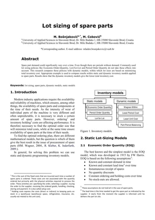
Inventory models
Static models
Dynamic models
Economic Order Quantity
Wagner-Within
Period Order Quantity
Least Period Cost
Lot for Lot
Least Unit Cost
Part-Period Balancing
Figure 1. Inventory models
2. Static Lot-Sizing Models
2.1
Economic Order Quantity (EOQ)
The best known and the simplest model is the EOQ
model, which was developed in 1915 by FW Harris.
EOQ is based on the following assumptions3:
Known and constant demand in time
Known and constant lead time4 over time
Instantaneous receipt of spares
No quantity discounts
Constant ordering and holding costs over time
No stock-outs are allowed.
3
4
These assumptions do not hold all in the case of spare parts.
The lead time is the time needed to get the spare part as indicated by the
supplier. It starts from the moment the supplier is informed until he
delivers the part on site.

2. It is necessary to know the following values for the
optimization:
D - Annual demand in units of the spare part
Cn - Fixed cost per order
h - Holding cost per unit per year
Optimal lot size is determined by the equation:
Q*
2.2
2 D Cn
h
(1)
Period Order Quantity (POQ)
The procedure of POQ model is following:
Calculate EOQ using average demand
Calculate time supply and round it to the nearest
integer
In each replenishment, order to cover that many
periods’ demand
Order interval is constant, but ordered quantities
could be different.
2.3
Lot-For-Lot Model (LFL)
Spare parts are ordered precisely when needed. Each
period is ordering a lot to satisfy only that period’s
demand. Lot-for-Lot is among the most popular with
practitioners since it is simple and produces the least
remnant work-in-process inventory. However, setup
costs can be excessive if too many small lot sizes result.
3. Dynamic Lot-Sizing Models
Dynamic lot-sizing models are used within the
demand which vary during a period of time.
Furthermore, all of the models described in this chapter
take assumptions:
Demand during period t is Pt and can be
anticipated.
Planning orders is done for a specific timetable
(planning horizons): t=1, 2... T
No shortage is allowed.
No limitations in warehouse nor in ordered
quantity.
The time necessary for the order realization is
ignored (equals zero) or it is constant
Warehouse expenses depend upon the level of
supplies at the beginning of a period.
The cost of ordering Cn, and holding costs ht,
Model objective is to determine the quantity of
ordering xt that minimize the inventory cost
during T periods.
In addition, it is supposed that the following data is
known:
Pt - Demand by periods
Cn(t) - The ordering cost (usually Cn(t)=const.=Cn)
ht - Inventory holding cost per unit (for unit that
remain at the end of a period t)
T - Analyzed number of periods (usually it is 12
months  T=12, i.e. one year)
Mathematical definition of the problem:
TCt*- Cost of an optimal ordering plan for the first t
periods
Zm,t - The cost of satisfying demands in periods m to t
by ordering in period m for the periods up to t.
Ym,t - The cost of satisfying demands for periods
1 to t:
• By having in mind the optimal ordering
plan in periods 1 to m-1
• Ordering in period m ( m t ) for periods m
to t
*
Ym,t TCm
TCt*
1
Z m ,t
min(Ym,t )
(2)
(1 m t )
(3)
Boundary conditions:
Ordering is performed only when the inventory
level is zero,
Ordered quantity exactly corresponds to the
demands in observed time periods,
State of supplies x ordered quantity = zero
The following means that is never optimal to
order if there are any quantity on stock,
If it is optimal to order in the period m to satisfy
the demand for periods m to t, it is also optimal
to order in the period m for the periods (m, m+1,
…., t).
Horizon theorem:
If it is in solving t periods optimal to order in the
period m to meet the demand in the period t, then in
resolving w periods (w>t) it is optimal to deliver order
in the period m or later:
If zt*=1 for the t period than zt*=1 for w periods
(w>t) and the ordering plan for the period t
remains unchanged (frozen)
If zt*=0 for t periods then zt*=0 or 1 for w
periods (w>t)

3. where zt* is a binary variable (= 1 if the order is issued
in period t, otherwise = 0)
3.1
Wagner-Within Model (W-W)
The goal of this model is to determine the
replenishment plan so that the ordering and holding
cost for certain period is minimal. Thus, the WagnerWhitin model for Zm,t and Ym,t takes the total inventory
cost.
The optimal ordering plan procedure is as follows:
a) Try to set inventory status demand to zero at the
beginning and end of the period T , i.e. I1=0 and
IT+1=0
b) Start with the first period i.e. t=1.
All demand must be satisfied  z*= (1,-,-,…,-).
Calculate TC1*=Y1,1=Z1,1=Cn
c) Setup t=t+1. If t >T End of procedure.
*
d) Calculate Ym ,t TC m 1 Z m ,t for all m which
correspond to unfrozen zm
e) Calculate TCt* min( Ym,t ), m t , and try to
determine z*=(z1*,…,zt*)
f) If zt*=1, frozen z* for the period (z1*,…,zt*)
g) Return to the item c)
Efficient computer implementation of the algorithm
was presented in 1985 by James R. Evans.
3.2
Least Period Cost Model (LPC)
Whenever the demand is positive model find the
order size that will cover the next "n" periods, where
"n" is set to minimize the average cost per unit time.
(E. Silver, H. Meal, 1973.)
The optimal ordering plan procedure is as follows:
a) Let the current period be t=1. For t=1, 2,…, T
calculate average ordering and holding cost, if
all items are ordered in the period t :
ACt
1
Cn
t
3.3
Least Unit Cost Model (LUC)
Whenever the demand is positive model find the
order size that will cover the next "n" periods, where
"n" is set to minimize the average ordering and holding
cost per unit. The procedure for finding the optimal
ordering plan in the period t=1, 2,…, T is as follows:
a) Let the current period be t=1. For t=1,2,…,T
calculate the average ordering and holding cost
per quantity unit, if all items are ordered in the
period t:
1
UCt
t
P
2
h
(4)
u 2
where ACt is the average setup and holding cost per
time unit (monthly) and Pτ is the demand in period τ.
b) Select the period t in which t is ACt < ACt+1.
That period should be noted as the period t*.
c) Order in period 1 for the period t*.
d) Subtract t* from the T and repeat the process
from the beginning
P
2
P
(5)
h
u 2
Where:
UCt - Average ordering and holding cost of
inventory per quantity unit.
Pτ - The demand in period τ
b) Select the period in which t is UCt<UCt+1.
Which we denote as period t*.
c) Order the required quantity for the period 1 up
to t*.
d) Repeat the procedure for the period t=t*+1,
t*+2, t*+3, …,T
3.4
Part-Period Balancing Model (PPB)
The basic idea of this model is to equalize the
holding cost in the period 1 to t with the cost of
ordering during the period 1 (U. Wemmerlov, 1983.).
The optimal ordering plan procedure is as follows:
a) Let the current period be t=1. Then calculate
holding cost for t=1, 2,…, T if ordering for
periods 1 to t is done in period t:
t
PPC t
P
2
t
t
Cn
h
(6)
u 2
b) Select a value for t that is PPCt closest to the
value of the setup cost Cn. Denote this period t*.
c) Order the required amount for the period 1 to t*.
d) Repeat the procedure for the period t=t*+1,
t*+2, t*+3, …,T
4. Ordering plan calculation
4.1
The input data
Spare parts demand often tends to be "lumpy," that
is, discontinuous and no uniform, with periods of zero

4. demand. According this assumption appropriate test
data are used in evaluation of certain inventory models.
Table 1. The spare part demand
Period
1
2
3
4
5
6
7
8
9
10 11 12 Total
Demand 22 62 0 35 124 68 25 0 120 70 44 30 600
In this test ordering (setup) cost per order is 30,00 €
and holding cost per unit and period is 0,2 €.
4.2
The test results
The figures 2. to 9. show the calculation results of
the ordering plan for particular model. Calculation is
done according to given procedures.
All values in the figures are given in Euros (€).
Figure 4. Period order quantity lot sizes
Figure 2. Lot-for-lot lot sizes
Figure 5. Least unit cost lot sizes
Figure 3. Economic Order Quantity lot sizes
Figure 6. Part-period balancing lot sizes

5. 5. Conclusion
Spare parts demand tends to be "lumpy," that is,
discontinuous and no uniform, with periods of zero
demand.
In general, dynamic models give better result than
static models for approximately 20%. The results of
dynamic methods depend on the value and mutual
respect of input data, and especially about the
relationship between the ordering and holding cost.
However, as it is evidently from the example and
additional analysis, the best result in determining the
optimal lot size of spare parts gives Wagner-Whitin
method.
Figure 7. Least period cost lot sizes
Figure 8. Wagner-Within lot sizes
Figure 9. Comparison of the total cost
References
[1] HM. Wagner, Comments on “Dynamic version of
the economic lot-size model”. Management
Science, Vol. 50, No 12, December 2004, pp.
1775-1777
[2] S. Chand, “A note on dynamic lot-sizing in a
rolling horizon environment”. Decision Sciences,
Vol. 13, 1982, pp 113-119
[3] J.D. Blackburn, R. A. Millen, Heuristic lot-sizing
performance in a rolling schedule environment.
Decision Sciences, Vol.11, 1980, pp 691-701
[4] R. Kleber, K. Inderfurth, A Heuristic Approach for
Integrating Product Recovery into Post PLC Spare
Parts Procurement. Springer Berlin Heidelberg,
2009., ISBN 978-3-642-00141-3, pp. 209-214
[5] E. Silver, H. Meal, A heuristic for selecting lot
size requirements for the case of a deterministic
time varying demand rate and discrete
opportunities for replenishment. Production and
Inventory Management Journal, Vol. 14, No 2
1973., pp. 64–74
[6] U. Wemmerlov, The part-period balancing
algorithm and its look ahead-look back feature: A
theoretical and experimental analysis of a single
stage lot-sizing procedure. Journal of Operations
Management, Vol. 4, No 1, 1983., pp. 23–39
[7] James R. Evans, An Efficient Implementation of
the Wagner-Whitin Algorithm for Dynamic LotSizing. Journal of Operations Management, Vol. 5,
No. 2, , 1985., pp. 229-235