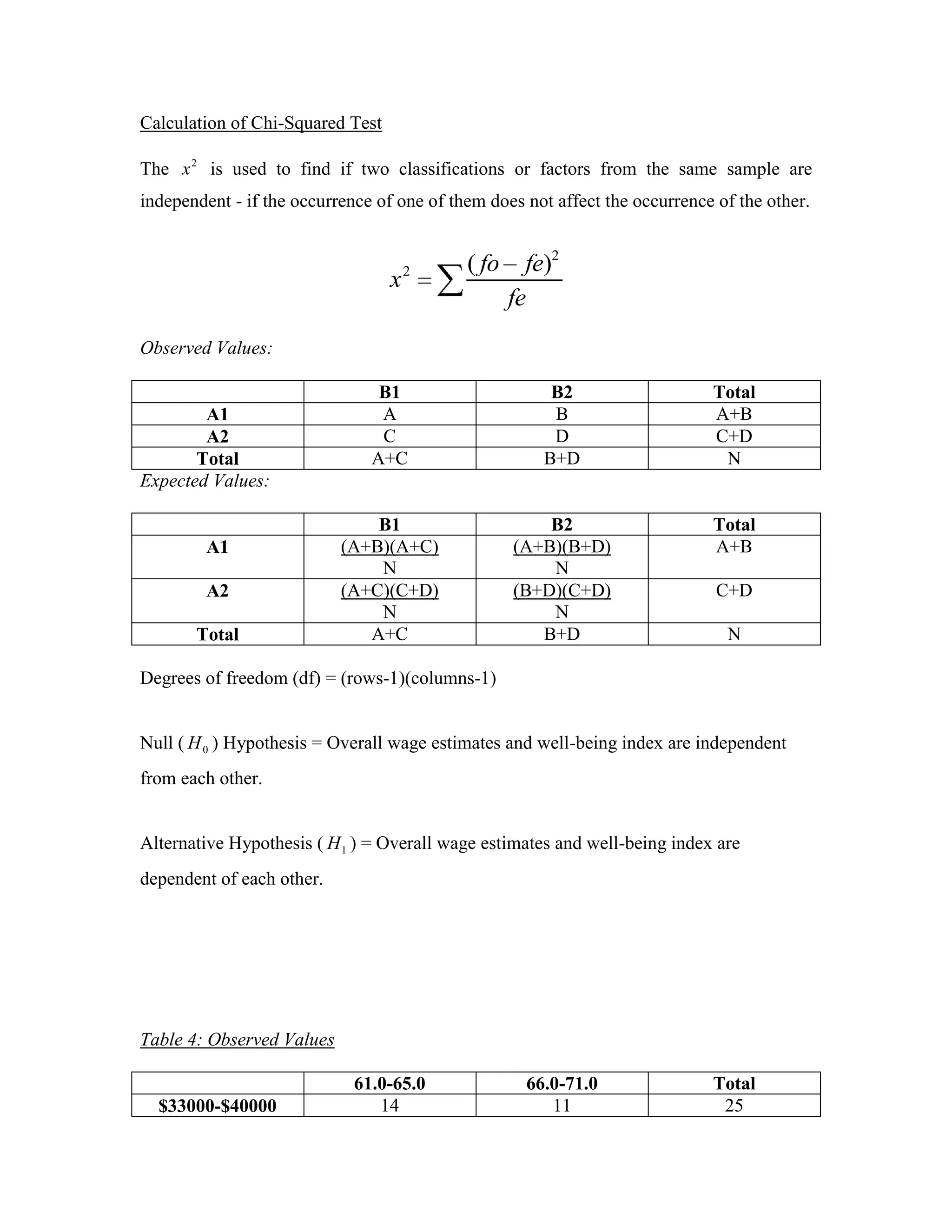
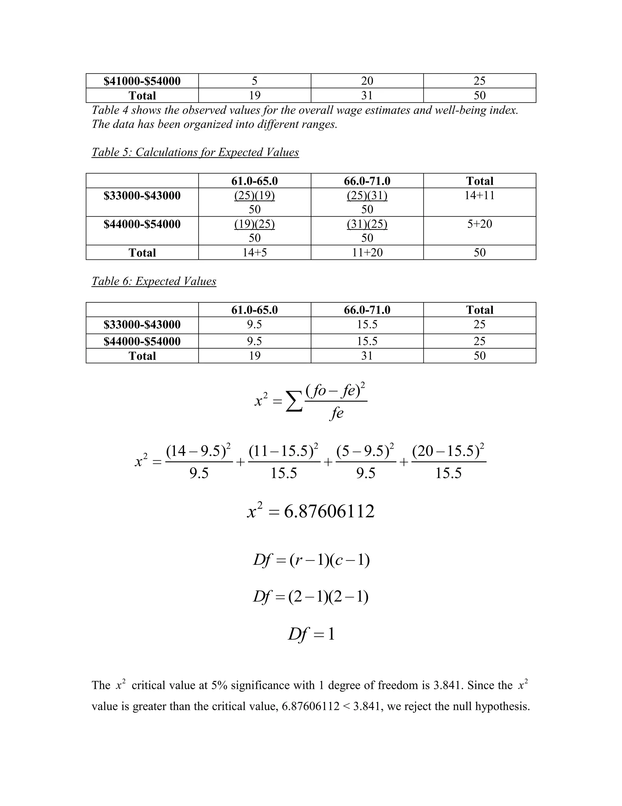
Calculation of Chi-Squared Test

The x 2 is used to find if two classifications or factors from the same sample are
independent - if the occurrence of one of them does not affect the occurrence of the other.


                                      2     ( fo     fe)2
                                  x
                                                   fe
Observed Values:

                                B1                      B2                   Total
        A1                      A                       B                    A+B
        A2                      C                       D                    C+D
       Total                   A+C                     B+D                    N
Expected Values:

                               B1                      B2                    Total
         A1                (A+B)(A+C)              (A+B)(B+D)                A+B
                               N                       N
         A2                (A+C)(C+D)              (B+D)(C+D)                 C+D
                               N                       N
       Total                  A+C                     B+D                      N

Degrees of freedom (df) = (rows-1)(columns-1)


Null ( H 0 ) Hypothesis = Overall wage estimates and well-being index are independent
from each other.


Alternative Hypothesis ( H 1 ) = Overall wage estimates and well-being index are
dependent of each other.


Table 4: Observed Values

                             61.0-65.0               66.0-71.0               Total
  $33000-$40000                 14                      11                    25
$41000-$54000                 5                     20                     25
       Total                   19                     31                     50
Table 4 shows the observed values for the overall wage estimates and well-being index.
The data has been organized into different ranges.

Table 5: Calculations for Expected Values

                             61.0-65.0                 66.0-71.0              Total
  $33000-$43000               (25)(19)                  (25)(31)              14+11
                                 50                        50
  $44000-$54000               (19)(25)                  (31)(25)              5+20
                                 50                        50
       Total                    14+5                     11+20                  50

Table 6: Expected Values

                             61.0-65.0                 66.0-71.0              Total
  $33000-$43000                 9.5                      15.5                  25
  $44000-$54000                 9.5                      15.5                  25
      Total                     19                        31                   50


                                      2     ( fo     fe)2
                                  x
                                                   fe

             2   (14 9.5)2      (11 15.5)2         (5 9.5)2        (20 15.5)2
         x
                    9.5            15.5              9.5              15.5

                                x2        6.87606112

                                 Df       (r 1)(c 1)

                                 Df       (2 1)(2 1)

                                          Df       1

The x 2 critical value at 5% significance with 1 degree of freedom is 3.841. Since the x 2
value is greater than the critical value, 6.87606112 < 3.841, we reject the null hypothesis.
We accept the alternative hypothesis, therefore, the overall wage estimates and the well-
being index are considered as not independent.

Sample of Math IA

  • 1.
    Calculation of Chi-SquaredTest The x 2 is used to find if two classifications or factors from the same sample are independent - if the occurrence of one of them does not affect the occurrence of the other. 2 ( fo fe)2 x fe Observed Values: B1 B2 Total A1 A B A+B A2 C D C+D Total A+C B+D N Expected Values: B1 B2 Total A1 (A+B)(A+C) (A+B)(B+D) A+B N N A2 (A+C)(C+D) (B+D)(C+D) C+D N N Total A+C B+D N Degrees of freedom (df) = (rows-1)(columns-1) Null ( H 0 ) Hypothesis = Overall wage estimates and well-being index are independent from each other. Alternative Hypothesis ( H 1 ) = Overall wage estimates and well-being index are dependent of each other. Table 4: Observed Values 61.0-65.0 66.0-71.0 Total $33000-$40000 14 11 25
  • 2.
    $41000-$54000 5 20 25 Total 19 31 50 Table 4 shows the observed values for the overall wage estimates and well-being index. The data has been organized into different ranges. Table 5: Calculations for Expected Values 61.0-65.0 66.0-71.0 Total $33000-$43000 (25)(19) (25)(31) 14+11 50 50 $44000-$54000 (19)(25) (31)(25) 5+20 50 50 Total 14+5 11+20 50 Table 6: Expected Values 61.0-65.0 66.0-71.0 Total $33000-$43000 9.5 15.5 25 $44000-$54000 9.5 15.5 25 Total 19 31 50 2 ( fo fe)2 x fe 2 (14 9.5)2 (11 15.5)2 (5 9.5)2 (20 15.5)2 x 9.5 15.5 9.5 15.5 x2 6.87606112 Df (r 1)(c 1) Df (2 1)(2 1) Df 1 The x 2 critical value at 5% significance with 1 degree of freedom is 3.841. Since the x 2 value is greater than the critical value, 6.87606112 < 3.841, we reject the null hypothesis.
  • 3.
    We accept thealternative hypothesis, therefore, the overall wage estimates and the well- being index are considered as not independent.