A simple explanation of the Hidden Markov Model

1. Hidden Markov
Model
Nghia Bui
Nov 2016
Andrei Markov (1856-1922)

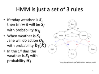
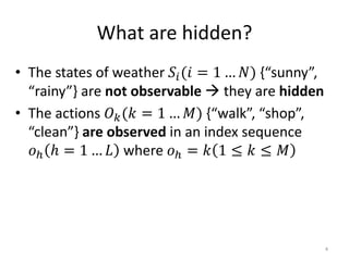
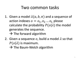
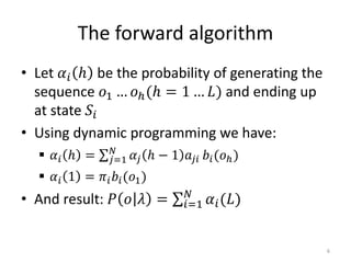
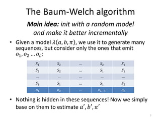
2. The weather problem
• I talked to Jane for 𝐿 days through telephone.
Everyday she told me what she does, either
“walk” or “shop” or “clean”, only one!
• I know, on a day, the weather in her city can
be either “sunny” or “rainy”, only one!
• But she didn’t tell me exactly the weather on
the 𝐿 days, and how it affected her actions.
• Then I have to figure out by myself!  HMM
2

3. HMM is just a set of 3 rules
• If today weather is 𝑺𝒊
then tmrw it will be 𝑺𝒋
with probability 𝒂𝒊𝒋
• When weather is 𝑺𝒊
Jane will do action 𝑶 𝒌
with probability 𝒃𝒊(𝒌)
• In the 1st day, the
weather is 𝑺𝒊 with
probability 𝝅𝒊
3
https://en.wikipedia.org/wiki/Hidden_Markov_model

4. What are hidden?
• The states of weather 𝑆𝑖(𝑖 = 1 … 𝑁) {“sunny”,
“rainy”} are not observable  they are hidden
• The actions 𝑂 𝑘(𝑘 = 1 … 𝑀) {“walk”, “shop”,
“clean”} are observed in an index sequence
𝑜ℎ ℎ = 1 … 𝐿 where 𝑜ℎ = 𝑘 1 ≤ 𝑘 ≤ 𝑀
4

5. Two common tasks
1. Given a model 𝜆(𝑎, 𝑏, 𝜋) and a sequence of
action indexes 𝑜 = 𝑜1, 𝑜2 … 𝑜 𝐿 please
calculate the probability 𝑃(𝑜|𝜆) the model
generates the sequence.
 The forward algorithm
2. Given a sequence 𝑜, build a model 𝜆 so that
𝑃(𝑜|𝜆) is maximum.
 The Baum-Welch algorithm
5

6. The forward algorithm
• Let 𝛼𝑖 ℎ be the probability of generating the
sequence 𝑜1 … 𝑜ℎ(ℎ = 1 … 𝐿) and ending up
at state 𝑆𝑖
• Using dynamic programming we have:
 𝛼𝑖 ℎ = 𝑗=1
𝑁
𝛼𝑗 ℎ − 1 𝑎𝑗𝑖 𝑏𝑖(𝑜ℎ)
 𝛼𝑖 1 = 𝜋𝑖 𝑏𝑖(𝑜1)
• And result: 𝑃 𝑜 𝜆 = 𝑖=1
𝑁
𝛼𝑖(𝐿)
6

7. The Baum-Welch algorithm
• Given a model 𝜆 𝑎, 𝑏, 𝜋 , we use it to generate many
sequences, but consider only the ones that emit
𝑜1, 𝑜2 … 𝑜 𝐿:
Main idea: init with a random model
and make it better incrementally
𝑆1 𝑆2 … 𝑆2 𝑆1
𝑆2 𝑆2 … 𝑆1 𝑆1
… … … … …
𝑆1 𝑆1 … 𝑆1 𝑆2
𝑜1 𝑜2 … 𝑜 𝐿−1 𝑜 𝐿
• Nothing is hidden in these sequences! Now we simply
base on them to estimate 𝑎′, 𝑏′, 𝜋′
7

8. Estimate 𝑎′, 𝑏′, 𝜋′
• To estimate 𝑎′𝑖𝑗, count the transitions from 𝑆𝑖 to
𝑆𝑗 and to other states
• To estimate 𝑏′
𝑖(𝑘), count the appearances of 𝑆𝑖
that have action index 𝑜ℎ = 𝑘, also count all the
appearances of 𝑆𝑖
• To estimate 𝜋′𝑖, count the appearances of 𝑆𝑖 at
the first element of all sequences, and count the
number of all sequences too
• But, to count all of things above, we need …
8

9. Forward and backward variables
• Using the forward algorithm we have 𝛼𝑖 ℎ
• Using the backward algorithm we have 𝛽𝑖 ℎ
the probability of generating the sequence
𝑜ℎ+1 … 𝑜 𝐿(ℎ = 1 … 𝐿) starting from tmrw,
given the state 𝑆𝑖 of today. Dynamic
programming is used again:
 𝛽𝑖 ℎ = 𝑗=1
𝑁
𝑎𝑖𝑗 𝑏𝑗(𝑜ℎ+1)𝛽𝑗 ℎ + 1
 𝛽𝑖 𝐿 = 1
9

10. Estimate 𝑎′
• Count transitions from 𝑆𝑖 to 𝑆𝑗:
𝜉𝑖𝑗 =
ℎ=1
𝐿−1
𝛼𝑖(ℎ)𝑎𝑖𝑗 𝑏𝑗(𝑜ℎ+1)𝛽𝑗(ℎ + 1)
• Thus:
𝑎′𝑖𝑗 =
𝜉𝑖𝑗
𝑘=1
𝑁
𝜉𝑖𝑘
10

11. Estimate 𝑏′
• Count the appearances of state 𝑆𝑖:
ℎ=1
𝐿
𝛼𝑖 ℎ 𝛽𝑖 ℎ
• Thus:
𝑏′
𝑖 𝑘 =
ℎ=1,𝑜ℎ=𝑘
𝐿
𝛼𝑖 ℎ 𝛽𝑖 ℎ
ℎ=1
𝐿
𝛼𝑖 ℎ 𝛽𝑖 ℎ
11

12. Estimate 𝜋′
• Count the appearances of 𝑆𝑖 at the first element:
𝛼𝑖 1 𝛽𝑖 1
• Count the number of all sequences:
𝑃 𝑜 𝜆 =
𝑖=1
𝑁
𝛼𝑖 𝐿
• Thus:
𝜋′𝑖 =
𝛼𝑖 1 𝛽𝑖 1
𝑃 𝑜 𝜆
12

13. Thank you!
• Contact: katatunix@gmail.com
13