
Recommended
Recommended
More Related Content
Similar to Running Head AZEOTROPIC EQUILIBRIUM AZEOTROPIC EQUILIBRIUM.docx
Similar to Running Head AZEOTROPIC EQUILIBRIUM AZEOTROPIC EQUILIBRIUM.docx (20)
More from healdkathaleen
More from healdkathaleen (20)
Recently uploaded
Recently uploaded (20)
Running Head AZEOTROPIC EQUILIBRIUM AZEOTROPIC EQUILIBRIUM.docx
- 1. Running Head: AZEOTROPIC EQUILIBRIUM AZEOTROPIC EQUILIBRIUM 2 Predicting Azeotropic Batch Distillation Equilibrium conditions Jassim Alajmi November 12, 2019 Jassim Alajmi, Ashraf Al Shekaili, and David Luong ChE 450 Group Number 5 Dr. Larry Jang California State University-Long Beach Department of Chemical Engineering Table of contents: 1. Abstract 1. Introduction 1. Materials and methods 1. Results 1. Dissections 1. Conclusion 1. References Abstract Vapor liquid equilibrium is very important now a days where
- 2. most separation plants uses it. It helps to separate gas from liquid or liquid from gas to use it for some other purpose. In this experiment the goal was to Predict VLE of non-ideal mixture of water and 2-propanol at atmospheric pressure. Additionally, the group focus on Find the relationship between batch distillation and VLE. The results were satisfying where the data that was collected where converted to a point in the that was under equilibrium curve. Introduction The vapor liquid equilibrium (VLE) is very important in chemical engineering field where it relate the distribution of a chemical species among the vapor phase and a liquid phase. Batch distillation is one of the essential processes in chemical engineering field nowadays, where it refer to the use of distillation column in order to separate mixture components into fraction of that mixture. The goal of this lab exercise is to study and analyze the conditions necessary for the azeotropic conditions which include but not limited to, bubble point, VLE composition and dew point. The name given to the liquid whose physical characteristics include boiling at a given composition and at a constant temperature is azeotrope. In this lab exercise, a mixture of water and 2-propanol was used as the specimen to evaluate the hypothesis when using batch distillation method (Gorak, 2014). This type of distillation has its applications in water treatment plants. It is also a common process used to perform separation of various materials in pharmaceutical plants. These, among other applications, makes this process very important in daily application. On the sections that follows, the list of equipment, materials, results and discussions are well explained. All the tests were carried out at normal atmospheric pressure. Enthalpies of mixing for such system has been reported before. The extensive knowledge obtained from testing the vapor-liquid equilibria in a water-n-propanol can be used for further testing of equilibrium systems such as the vapor-liquid equilibria in water-n-propanol- n-butanol system (Gunawan, 2010).
- 3. Below are some of the important equations that shall be used when performing the analysis of the results obtained experimentally. The Antoine equation . .. . . . . . . . . . . . . . . . . . . . . . . . . . . .. . . … . . . . . . . . . . . . . . .Equation 1 Where i= 1,2. At point 1, the saturation pressure of 2-proponol is obtained while at point 2, the saturation pressure of 2- propanol is obtained. . . . . . . . . . . . . . . . . . . . . . . . . .. . . . . . . . . . . . . . . . . . . . Equation 2 When the value of x and y in the equation 2 above are equal azeotropic point is achieved, it is the point where the mole fraction of the liquid and the gas are equal. It follows then that the Raoult`s Law is as follows; . . . . . . . . . . . . . . . . . . . . . . . . .. . . . . . . . . . . . . . . . . . . . Equation 3 When x=y, the values ( activity coefficient) can be obtained. Material and method Apparatus i. Boiling chips ii. Boiling flask iii. Electronic balance iv. Othmer still distillation apparatus v. Refractometer vi. Heating mantle vii. Beakers/ vials viii. Condensers Procedure The binary mixture shouldn’t, under any circumstance be drunk by students whether in lab or anywhere else. It was also necessary that students worn safety goggles and lab coat to protect them in case the mixture ever flashed while carrying out the experiment. Students were also advised to not spill any
- 4. liquid on electrical equipment to avoid damaging it and also to prevent electrocution. It was also important for student to note that other than being highly flammable liquid, isopropanol was capable of causing eye irritation (Cunningham, 2011). i. The batch distillation was set up as shown in the figure and the reflux turned on. The following ratios were used for water and 2-propanol during the experiment, 10%, 15% and 20%. A 100g of the solution was used during the experiment. Figure 1: The distillation set up for the lab exercise Figure 2: The actual lab set up for the distillation ii. the mixture was weighed on the electronic balance after which it was poured into the boiling flask. A beaker was placed on the electronic balance where the distillate would pour. The balance was first zeroed to avoid errors during the measurements. The refractometer was zeroed using the DI water. The reflective index of the initial mixture was obtained so that the mass fraction of the 1- propanol could be obtained (Kagaku , & Kōgakkai , 2018). iii. The mixture was heated. The reflective index of the mixture heated was recorded after every degree rise in temperature. The refractive index pf the distillate was also obtained. iv. The process continued until the weight percent of the alcohol vapor ran out. Results Parameters for equations 1, 2 and 3 obtained from the experiment. Van Laar 2.470754 1.090241 Table 1: Equation parameters
- 5. 1.075009 2.115062 0.6813 0.3187 Run 1 : not adding anything Time (s) Condensate wt % 2-propanol mol % Pool wt % mol % 0 1.37021 1.3626 180 1.37062 1.36286 360 1.3716
- 6. 1.35401 540 1.37133 1.36284 720 1.37146 1.36138 1005 1.37167 1.36261 1200 1.37194 60.73846 0.3168695 1.36255 36.82 0.14874552 Table 2: The model parameter results Table 3:The refractive index to wt% 2-propanol
- 7. Run 2 : adding 2-Propnol Time (s) Condensate wt % 2-propanol mol % Pool wt % mol % 0 1.36799 1.36276 180 1.37072 1.3627 360 1.37121 1.36259 540 1.37116
- 8. 1.36266 720 1.3712 1.36261 900 1.37147 59.2333 0.30345284 1.36249 36.58 0.14744214 87.7 0.68130923 0.31869077 Table 4: Run 2 mole fraction of the water and wt% 2-propanol Run 3 : adding water
- 9. Time (s) Condensate wt % mol % Pool wt % mol % 0 1.34096 1.36219 180 1.34096 1.36215 360 1.34096 1.36234 540 1.34107
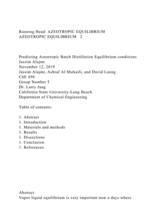
- 10. 1.3621 720 1.34147 1.3623 900 1.34179 9.79 0.03151387 1.36228 36.16 0.14517535 Table 5: Run 3 mole fraction of the water and wt% 2-propanol Discussion The following graphs were obtained when Van Laar model was used. The liquid composition of the liquid is in the x-axis and vapor composition is in the y-axis. Figure 3: The graph above is a vapor-Liquid equilibrium diagram developed using the Van Laar model Figure 4: The bubble point and dew point diagram for the parameters predicted using the Van Laar Model Table 1 indicate and where they are the parameter for the Van
- 11. Larr equation which they been used to find model parameter for azeotropic condition. Table 2 indicate the model parameter that was obtained. Table 3-5 are the three trials that was done in the experiment. Trial one was without adding anything to the apparatus, trial two wad run by adding 2-propanol, and trail 3 was done by adding water and the date shown in the table was obtained. The refractive indices and densities of the binary system were recorded in the table 4 at room temperature (Nevers, 2013). The excess volumes of mixing the binary system have been calculated from the densities recorded before used to plot the figure 4 above. The asymmetry seen in the curve is probably not real at all since many thermodynamic functions are not asymmetric at all. The tables 4 and 5 contain the equilibrium results for the water-n-propanol system. The absolute deviation of the above values from smooth curve is probably less than 0.001. it was also found that from the curves plotted. ===.. At low alcohol concentration, there challenges encountered when operating the equilibrium because the boiling region did rapidly change. The graphical boiling point values for n-propanol and water through extrapolation in a t-x diagram at 760 mm Hg are 97.1 and 100. respectively. The values differ from those obtained through Antoine equations which were 97.1and 100.00 respectively. The estimated errors from the extrapolation process is approximately 0.C. Conclusion The lab exercise was success because the state objective was achieved. The conditions necessary for azeotropic equilibrium were determine. For this type of equilibrium to take place the mole ratio of the vapor and liquid propanol must be equal. Other than plotting several figures which assisted in analysis, several other equations were introduced in the process which were used to validate the results obtained from the experiment. Batch distillation methods gives results with a higher degree of accuracy compared to other methods of distillation. The conditions for processing the type of feeds involved helped in the analysis of the product. This method is useful in
- 12. pharmaceutical process because the exact ratio and quantities are needed when developing certain drugs whose components can prove lethal if they are used in excess. Though the errors were minimal during the experiment, the possible sources of errors could be failure to zero the electronic balance and thereby false values of mass were obtained. When determining the ratio of water and propanol, it was possible some errors occurred and thereby falsifying the results (Rousseau, 2017). References Gorak, A. (2014). Distillation: Fundamentals and Principles. Academic Press. Kagaku Kōgaku Kyōkai (Japan), & Kagaku Kōgakkai (Japan). (2018). Journal of chemical engineering of Japan. Tokyo: Society of Chemical Engineers, Japan. Rousseau, R. W. (2017). Handbook of separation process technology. New York: John Wiley & Sons. Nevers, N. . (2013). Physical and chemical equilibrium for chemical engineers. Hoboken, N.J: Wiley. Gunawan, R. J. (2010). Experimental measurement of liquid- fluid equilibria of dodecane + carbon dioxide and methyl oleate + carbon dioxide. Cunningham, J. R., & Jones, D. K. (2011). Experimental results
- 13. for phase equilibria and pure component properties. New York, N.Y: American Institute of Chemical Engineers X-Y Plot for IPROPNOL and H2O (Thermo = VANL01, P = 14.696 psia) x = y0101Equilibrium curve05.0000001000000002E- 20.10.150000009999999990.20.250.300000009999999980.3499 99989999999980.400000010000000020.449999990000000020.5 0.550000009999999980.600000019999999970.64999998000000 0030.699999990000000020.750.800000009999999980.8500000 19999999970.899999980000000030.94999999000000002100.40 5796800000000010.495240720000000020.52741735999999995 0.541687490000000050.549796219999999950.55638145999999 9990.563598449999999970.572563830.583924530.5981140099 99999970.615481020000000050.636362850000000040.6611318 60000000020.690232040000000050.724213180000000010.7637 69570000000010.809788469999999980.863416250.9261524100 00000040.99998719000000003 Liquid Composition, Mole Fraction IPROPNOL Vapor Composition, Mole Fraction IPROPNOL set of calculated data have been filed with the ACS Mi- crofilm Depository Service. Nomemclature GE = excess Gibbs free energy, cal/g-mol x1 = mole fraction of the more volatile component of a y1 = mole fraction of the more volatile component of a y1,yz = activity coefficients for components 1 and 2 in q h , $ ~ = coefficient of correction for nonideality of the
- 14. T = total pressure, m m Hg binary mixture in the liquid phase binary mixture in the vapor phase the liquid phase vapor phase for components 1 and 2 Literature Cited (1) Minh, D. C.. MS thesis, Sherbrooke University, Sherbrooke. Que., Canada (1970). (2) Minh, D. C., Ruel, M., Can. J . Chem. Eng.. 4 8 , 501 (1970). (3) Minh, D. C.. Ruel, M.,ibid., 49, 159 (1971). ( 4 ) Prengle. H . W., Palm, G. F., ind. Eng. Chem., 49, 1769 (1957). (5) Ramalho, R . , Delmas, J.. Can. J . Chem. Eng., 46, 32 (1968). (6) Ramalho, R., Delmas, J., J . Chem. Eng. Data, 1 3 , 161 (1968). (7) Selected Values of Properties of Chemical Compounds. Thermody- namics Research Center, Texas ABM University, College Station, Tex., 1970. Received for review January 19. 1971. Resubmitted February 10, 1972. Accepted October 26, 1972. Grants from the National Research
- 15. Council of Canada are gratefully acknowledged. Additional data will appear fol- lowing these pages in the microfilm edition of this volume of the Journal. Single copies may be obtained from the Business Operations Office, Books and Journals Division. American Chemical Society, 1155 Sixteenth St., N.W., Washington, D.C. 20036. Refer to the following code number: JCED-73-41. Remit by check or money order $7.00 for photocopy or $2.00 for microfiche. Vapor-Liquid Equilibria in Mixtures of Water, n-Propanol, and n-Butanol Richard A. Dawe,’ David M. T. Newsham,2 and Soon Bee Ng Deoartment of Chemical Enoineerino, Universitv of Manchester Institute of Science and Technology. Manchester, M60 lob, U . K . Measurements of vapor-liquid equilibria in the systems water-n-propanol and water-n-propanol-n-butanol at atmospheric pressure are reported. The results for the ternary system have been compared witb those predicted from the binary mixtures using the equation of Renon and Prausnitz. Agreement is very satisfactory. Densities and refractive indices of the binary and ternary mixtures at 25°C are also reported and the excess volumes of binary mixing have been calculated. This paper reports the results of measurements of vapor-liquid equilibria for the systems water-n-propanol and water-n-propanol-n-butanol at atmospheric pres-
- 16. sure. Enthalpies of mixing for these systems have pre- viously been reported (5, 6) and liquid-liquid equilibrium studies have also been published ( 7 0 ) . Vapor-liquid equilibria in the system water-n-propanol have been extensively investigated ( 7 ) and this system is therefore suitable for testing the performance of the equi- librium still used in the present work. No measurements of vapor-liquid equilibria in the system water-n-propanol- n-butanol have previously been reported. Experimental Materials used in this investigation were purified as de- scribed in ref. 5 and 6. For the measurements of vapor-liquid equilibria, an equilibrium flow still similar to that described by Vilim et at. (74) was constructed. This instrument has the advan- tage that it avoids recirculation of the condensed vapor, which enables reasonably precise results to be obtained in a short time (15 min). The still used in this work dif- fered from that of Vilim et al. in that the thermometer well was designed to accommodate a 50-ohm capsule- type platinum resistance thermometer (Rosemount Engi- neering Co. Ltd.) and the vacuum jacket that insulated the equilibrium chamber was extended to include the droplet separator (Figure 1 ) in order to minimize thermal I ‘I 1 I ’Present address, Department of Chemical Engineering,
- 17. University of Leeds, Leeds, U.K. To whom correspondence should be addressed. Figure 1. Equilibrium chamber of the flow still A, thermometer weli; B, vacuum jacket; C, droplet separator; D, to vapor condenser; E, 3-mm capillary; F, to liquid cooler; G, Cottrell pump; H, boiler; J. float-valve; K , reservoir 44 Journal of Chemical a n d Engineering D a t a , Vol. 18, No. 1, 1973 losses. The platinum thermometer was calibrated by intercomparison with a 25-Ohm platinum thermometer that had been calibrated at the National Physical Labora- tory (U.K.) on the International Practical Temperature Scale of 1948. Resistances were measured by potentio- metric comparison with a 100-ohm standard resistor on a vernier potentiometer (H. Tinsley and Co. Ltd., U.K.). Temperatures could be measured to within f0.02"C with the platinum thermometer. No attempt was made to con- trol the pressure in the equilibrium still, but the pressure in the laboratory was measured by a mercury manometer and cathetometer with an accuracy of f 0 . 0 5 mm Hg. All pressures were corrected to give the equivalent height of a mercury column at 0°C and standard gravity. For this purpose a value of the local acceleration due to gravity of 981.370 f 0.001 c m s e c - 2 was used. Preliminary measurements in which pure water was boiled in the still showed that thermal equilibrium could
- 18. be attained in it to within 0.02"C. Subsequent experi- ments with water and n-propanol mixtures indicated also that transfer of material between vapor and liquid phases was sufficiently rapid for a reasonable approach to equi- librium conditions to be made. The ratio of liquid to vapor flow rates was, typically, about 10. The droplet separator functioned satisfactorily throughout the measurements and no indications of entrainment in either vapor or liquid phases were observed. The liquid samples were always used in the freshly distilled state since they were contin- ually recycled through the still. Compositions of the binary liquid mixtures were deter- mined by measurement of their refractive indices, and those of the ternary mixtures were deduced from density and refractive index measurements. A dipping refractom- eter that was equipped with thermoprisms (Carl Zeiss, Jena) and which had a measuring precision of f 2 X was used. The temperature of the prisms was con- trolled at 25.00" f 0.05"C by circulating water from a thermostat. Illumination was provided by a sodium lamp. Densities were measured at 25°C using 5-cm3 Lipkin pycnometers that had been calibrated with distilled water. The density of water at 25°C was taken to be 0.99705 gram ~ m - ~ . The precision of the density mea- surements was estimated to be f0.0002 gram ~ m - ~ . Calibration curves for composition as a function of densi- l o o P,.,* / 6 0 w* 4 0
- 19. 2 0 0 20 40 6 0 80 Wl Figure 2. Curves of constant density and refractive index for water (1)-n-propanol (2)-n-butanol (3) at 25°C ty and refractive index were prepared by measuring these properties for samples of known composition. For esti- mating ternary compositions it was necessary to prepare curves of constant density and refractive index as a func- tion of composition. This was achieved by interpolating the primary results graphically to give the curves of Fig- ure 2. The estimated errors in the measured mole fractions are different for each component. They are f 0 . 0 0 5 for water and fO.O1-0.05 for n-propanol and n-butanol. The reason for this is apparent on examination of Figure 2 which shows that the curves of constant density are al- most vertical straight lines. This means that the percent- age of water ( Wl) can always be accurately estimated because it is virtually independent of the angle at which the curves of constant density and refractive index inter- sect. The percentage of propanol ( WZ) is more difficult to determine particularly in the region 40 < W t < 60% where the density and refractive index curves are almost parallel to each other. The butanol composition (W3) is also subject to considerable uncertainty in this region. For values of W1 < 40%, however, W1 and W3 can be determined to within about 1%. Th'ese estimates of the uncertainties are substantiated in the comparison of ex-
- 20. perimental and calculated vapor compositions made later. Results and Discussion The densities and refractive indices for the three binary systems and the ternary system at 25°C are recorded in Table I. Table I I gives densities and refractive indices measured at 25.9"C for mixtures with compositions lying on the liquid-liquid phase boundary at 25°C. The excess volumes of mixing for the three binary sys- tems have been computed from the densities and are re- corded in Figure 3. The vertical error bars for the n-pro- panol-n-butanol system represent an uncertainty in the density measurements of f 0 . 0 0 0 2 gram ~ m - ~ . The ap- parent asymmetry is probably not real. The other excess thermodynamic functions are not asymmetric (6). Vapor-liquid equilibrium results for the systems water- n-propanol and water-n-propanol-n-butanol are present- ed in Tables I l l and I V , respectively. References to vapor-liquid equilibrium data for water-n-propanol may be / / -0 6 I x Figure 3. Excess volumes of mixing of water-n-propanol (0), water-n-butanol ( A ) , and n-propanol-n-butanol ( 0 ) at 25°C; x is the mole fraction of the second component Journal of Chemical and Engineering Data, Vol. 18, No. 1, 1973 45
- 21. Table I. Densities and Refractive Indices of Solution s of Water, Table 11. Refractive Indices and Densities of Mixtures of Water, n-Propanol, and n-Butanol at 25°C n-Propanol, and n-Butanol at 25.9'C and at Compositions Lying on the Binodal Curve at 25°C p l g r a y 7 W l W2 7 P I S cm-3 w1 wz w3 cm - 100 0 0 2.51 6.31 10.75 16.51
- 22. 22.69 30.96 41.08 55.05 72.93 0 0 0 0 0 0 0 0 0 2.32 5.27 9.06 13.55 18.89 93.85 94.64 96.96 98.37
- 32. 1.39342 1.39004 1.38995 1.38129 1.38225 1.38352 1.38476 1.38000 1.37758 1.37546 1.37251 1.37090 1.36398 1.36230 1.35149 i 3 3 8 0 1 21.6 7.7 1.38609 0.84643 31.4 23.4 1.37931 0.86490 40.5 27.2 1.37395 . . . 55.6 25.2 1.36465 . . . 72.5 16.4 1.35290 . . . 77.8 13.6 1.35085 0.95925 80.8 11.9 1.34870 0.96558
- 33. Table Ill. Vapor-Liquid Equilibrium Data for Water (1)- n-Propanol (2) P, m m H g t , O C x 2 Y2 71 Y2 ' 756.33 756.73 756.73 756.73 756.07 755.86 757.97 757.97 757.97 758.08 758.08 758.08 756.33 759.13 759.13 759.13 98.18 96.47
- 37. 1.593 1.519 1.260 1.051 1.032 0.998 0.994 0.994 where difficulties are encountered in qperating an equilibri- um still because of the rapid change of boiling point with composition in this region. The boiling points of pure water and n-propanol obtained by extrapolation of the t - x diagram, after correction to 7 6 0 m m Hg, were 100.03" and 9 7 . 1 3 " C compared to values of 100.00" and 9 7 . 0 7 " C calculated from the Antoine equations of ref. 8. The esti- mated error on the extrapolated values of the boiling points is 0.1 "C. The validity of the results may also be checked by applying thermodynamic consistency tests to the liquid phase activity coefficients. The latter were calculated from the following equation which includes corrections for vapor phase nonideality:
- 38. y , = ( y , P / x , P P j exp [ ( B a t - V d ( P - P , " ) / R T ] (1) This equation assumes that the vapor phase behaves as an ideal solution. The reference state for the activity coefficients is the pure liauid at the temperature and total pressure of the soiution. The second virial coefficients for found in the compilation Of Hala et ( 7 ) ' For the pur- water and n-propanol were taken from the work of Collins pose of evaluating the performance of the equilibrium still used in the present investigation we have compared the data selected by Hala et al. (8) with our results in Figure and Keyes (') and ( 2 ) 7 respectively~ and the pure component vapor pressures were calculated from the An- toine equations given in ref. 8. The maximum value of the vapor phase correction was 1 . 5 % . The consistency test was applied by writing the Gibbs-Duhem equation in the form 4 which is a plot of vapor phase composition against liq- uid phase composition. The average deviation of the vapor compositions determined in this work from the smooth curve of Figure 4 is 0.001. We find, for the
- 39. azeotropic composition, y2 = x z = 0.433 compared to values of 0.432 and 0.426 given by Doroshevsky and Po- lansky (3) and Murti and Van Winkle ( 9 ) . At other com- positions the agreement is generally good; the largest de- viations (up to 0.04) occur at low alcohol concentrations 1n(YI/Y2)dxl - l:: j$ ( g ) , d x : - 0 ( 2 ) Figure 5 is a plot of In 73/72 against xl. The area ratio I A , / A 2 1 obtained by Simpson's rule integration is 0 . 9 7 5 . t - 0 46 Journal of Chemical and Engineering Data, Vol. 18, No. 1, 1973 Table IV. Vapor-Liquid Equillbrium Data for Wator (1) and n- Propanol (2)-n-Butanol (3) ~~ ~~ Exptl Calcd Eq 7 X 1 x 2 Y1 Yz Y1 Yz AYi AYZ AYJ P, rnrntig t , " C
- 48. 0.013 1 --- 1 0 0.2 0.4 0.6 OE 1.0 x2 Flgure 4. Equilibrium vapor and liquid compositions for water- n-propanol at atmospheric pressure 0 this work, A Doroshevsky and Polansky ( 3 ) . Murti and Van Winkle (9). This is satisfactory since the second term of Equation 2 has been neglected. However* this integral may be evalu- ated using the enthalpies of mixing of Plewes et al. ( 1 1 ) Figure 5. Plot of In ( y ~ / y * ) against XI for water (1)-n- propanol (2) at atmospheric DreSSure . .
- 49. and from values of ( a T / b x l ) p obtained by graphical dif- ferentiation of the t - x curve. When this is done the area ratio is increased to a value of 0.995. The corrected Prediction of Ternary Phase Equilibria curve cannot be shown with clarity in Figure 5 but the main differences occur for values of X I 0.2 and > 0.9 because of the high values of ( d T / a x l ) p in these regions. The closeness of the area ratio to unity confirms the thermodynamic consistency of our results. Figure 5 also indicates the high precision of the results for the water-n-propanol system, as does Figure 6 which is a plot of the excess Gibbs energy against x 2 . The results of the measurements on the ternary system are collected together in Table I V , and are discussed below. Jouri w Recently, Renon and Prausnitz (72) have proposed a method of evaluating the thermodynamic properties of multicomponent mixtures from a knowledge only of the properties of the appropriate binary pairs. The method is
- 50. particularly suitable for partially miscible systems. We have therefore applied it to the system water-n-propanol- n-butanol. According to Renon and Prausnitz the excess Gibbs free energy of a binary liquid mixture is given by the following Equation: G"RT - x l x ~ [ r 2 1 G 2 1 / ( x I + x&)+ rl2GI2/(x2 + x , ~ , , ) ] ( 3 ) 11 of Chemical and Engineering Data, Vol. 18, No. 1, 1973 47 Table V. Parameters of the Equation of Renon and Prausnitr for Binary Systems of Water ( l ) , n-Propanol (2), and n-Butanol (3) Figure 6. Plot of the excess Gibbs free energy against x 2 for water (1 )-n-propanol (2) at atmospheric pressure A I .o 0 0.1 0.2 0.3 0 x3 -
- 51. Figure 7. Projection of the phase diagram for water-n-propa- nol-n-butanol at 760 mm Hg -- vapor 3-phase curve, .... liquid 3-phase curves, - tie triangles, C critical point where 721 = ( 9 2 1 - g11)/RT, 7 1 2 = (912 - 922)/RT G21 =exp(-a21721), GIZ = e x p ( - a 1 ~ 7 1 ~ ) , a n d a 1 2 =(YZI. The quantities gi, are interaction energies and cy12 is the so-called "nonrandomness parameter. " The three in- dependent parameters of Equation 3 were obtained for the three binary systems by making a nonlinear least- squares fit to the excess Gibbs energies, assuming the parameters to be independent of temperature. The data for n-propanol-n-butanol and water-n-butanol were those of Gay ( 4 ) and Smith and Bonner ( 7 3 ) , respectively. The excess Gibbs energies for the system n-propanol-n-buta- no1 are much smaller than those of the other two systems and, within the experimental error, GE is a symmetrical function of composition. For this system, therefore, the parameter was taken to be zero when Equation 3 reduces to the second-order Margules equation: G' = 2 ~ 1 x 2 (gzi - gii) ( 4 )
- 52. The binary parameters are given in Table V . All of the 48 Journal of Chemical and Engineering Data, Vol. 18, No. 1, 0.4 A 0 ai 0.2 0.3 a4 a5 x3 - Figure 8. Isothermal sections (with tie-lines) of the phase di- agram for water-n-propanol-n-butanol at 89" and 91 OC --vapor curves, - liquid curves systems could be fitted to Equation 3 with root-mean- square deviations of less than 0.003 in G E / R T . The binary parameters were then used in Equation 5, which is the ternary form of the Renon-Prausnitz equa- tion, to calculate the activity coefficients of the ternary system and hence bubble point temperatures and vapor phase compositions at 760 m m Hg: where Gkk = 1 and 7kk = 0. The results of the calculations are given in Table I V
- 53. where the vapor phase compositions are compared with the experimental values. The agreement is very satisfac- tory, bearing in mind the limitations of the analytical method used for obtaining the compositions of n-propanol and n-butanol. Equation 5 has also been used to examine the phase diagram in the vicinity of the liquid-liquid region. I n an at- tempt to establish the liquid-liquid phase boundary and tie-lines by searching (graphically) for the compositions at which the activities of each component were uniform, it was found that the equilibrium compositions were too sensitive to small changes in the activity for a reliable estimate of the binodal curve to be made. Instead, esti- mates of the binodal curves at temperatures close to the bubble point were made by extrapolating the liquid-liquid equilibrium data previously reported ( 70). Liquid-liquid 1973 tie-lines were then obtained by finding the compositions at which curves of constant activity of n-propanol inter-
- 54. sected the binodal curve. The resultant liquid and vapor three-phase curves are shown, in projection, in Figure 7. The three-phase curves cover a range of boiling points of only about 3°C. The system does not form a ternary azeotrope, homo- geneous or heterogeneous. The vapor and liquid surfaces are rather flat, however, in the region between the homo- geneous water-propanol azeotrope and the heterogene- ous water-butanol azeotrope. This is evident on inspec- tion of two isothermal sections of the phase diagram at 89" and 91 "C, as shown in Figure 8. Acknowledgment We are grateful to G. L. Standart for his encourage- ment. We are also indebted to F. P. Stainthorp and H. M. Rash for their guidance in the preparation of the neces- sary computer programs. Nomenclature B i j = second virial coefficient, cm3 m o l - ' GE = excess Gibbs free energy of mixing, J mol G i j = parameter of Renon-Prausnitz equation g i j = parameter of Renon-Prausnitz equation
- 55. H E = excess enthalpy of mixing, J m o l - ' P = total pressure, m m Hg Pio = pure component vapor pressure, mm Hg R = gas constant, J K - ' mol-' T = Kelvin temperature, K t = Celsius temperature, "C V E = excess volume of mixing, cm3 mol - 1 x i = liquid phase mole fraction y t = vapor phase mole fraction W i = w t % - 1 Greek Letters aij = parameter of Renon-Prausnitz equation T i = liquid phase activity coefficient 7 = refractive index (sodium D-line) p = density, g ~ m - ~ T i j = parameter of Renon-Prausnitz equation Subscripts
- 56. 1 = water 2 = n-propanol 3 = n-butanol i , j , k , l , r = running variables Literature Cited Collins, S. C., Keyes, F. G., Proc. Amer. Acad. Sci., 72, 283 (1938). Cox, J . D., Trans. FaradaySoc., 57, 1674 (1961). Doroshevsky, A.. Polansky. E., Z. Phys. Chem.. 73,192 (1910) Gay, L., Chim. Ind. 18, 187 (1927). Goodwin. S. R . , Newsham, D. M. T., J. Chem. Thermodyn., 3 , 325 (1971). Goodwin, S. R . . Newsham, D. M. T., ibid., 4, 31 (1972). Hala, E., Pick, J., Fried, V., Vilim, O., "Vapour-Liquid Equilibrium," 2nd ed., p 404, Pergamon, London, 1967. Hala, E., Wichterle. I . , Polak, J., Boublik, T., "Vapour-Liquid Equi- librium Data at Normal Pressures," Pergamon, London, 1968. Murti. P. S., Van Winkle, M . , Ind. Eng. Chem., 3, 72 (1958). Newsham, D. M. T., Ng, S. E., J. Chem. Eng. Data, 17 (2), 205
- 57. Plewes. A. C., Jardine. D. A., Butler, R. M., Can. J. Technoi.. 32, Renon, H., Prausnitz, J. M., AlChEJ., 14, 135 (1968). Smith, T. E., Bonner, R. F., Ind. Eng. Chem., 41, 2867 (1949): Vilim, O., Hala, E., Pick, J., Fried, V.. Collect. Czech. Chem. Com- mun., 19, 1330 (1954). (1972). 133 (1954). Received for review March 30, 1972. Accepted August 21, 1972. S. B. Ng received financial support from the British Council. Integral Isobaric Heat of Vaporization of Benzene-I ,2=Dichloroethane System Yaddanapudi Jagannadha Rao and Dabir S. Viswanathl Department of Chemical Engineering, Indian Institute of Science, Bangalore- 72, India Integral isobaric heats of vaporization of benzene-l,2-
- 58. dichloroethane mixtures were measured at pressures of 684 and 760 mm of Hg using a modified Dana's apparatus. The results were found to be linear with composition. Latent heat of vaporization is a very important property needed in the design and operation of chemical plants. Several investigators have therefore devised methods for the determination of this property. Very little data ( 7 , 2, 6-70, 72, 73, 7 5 ) are available on heat of vaporization of mixtures. The first published work on latent heats of mixtures was by Dana (2) who worked at atmospheric pressure and cryogenic temperatures. Apart from other sources of error, the main source of error in his experimentation was ' To whom correspondence should be addressed due to heat leak because of the considerable tempera- ture gradient between the system and the surroundings. Subsequently, attempts have been made (6-70, 72, 73) to minimize the heat leak and reduce other sources of error involved. The best modification was due to Shettigar et al. (9) who introduced a liquid meter also to avoid
- 59. changes in the equilibrium condition of the experiment. Experimental Materials. Benzene used was of Pro analysi grade pro- duced by Sarabhai Merck Ltd., India, with a reported boiling range of 80-81°C. This material was subjected to the thiophene test. Thiophene was removed by treating it with concentrated sulfuric acid and distilling i t after sepa- ration and washing it with distilled water. Benzene then was dried over calcium chloride, filtered, and further puri- fied in a distillation column. Only the middle fractions of the distillate were collected. Table I gives a comparison of the experimentally determined physical properties with the literature values. Journal of Chemical and Engineering Data, Vol. 18, No. 1, 1973 49 GUIDE FOR THE PREPARATION OF REPORTS
- 60. This guide for the writing of laboratory reports is intended to help you write your reports and to understand the criticisms of them made by your instructors. You should study this guide before writing each report, review it before turning in each report, and use it to help interpret the criticism on reports returned to you. You write reports in this course not only to explain the experiments performed and what you learned from them, but also to learn, under the guidance of you instructors, something about the kind of writing you will be expected to do as an engineer. Engineers write many kinds of reports. Some of these, perhaps most, may be called routine reports, involving the filling in of blanks in a report sheet, or the supplying of tables, graphs, or drawings, with perhaps only a few sentences of explanation here and there. The routine report is read by those are closely familiar with the writer’s work. They know what to look for and want facts quickly;
- 61. hence elaborate introductions, transitions, and explanations are usually unnecessary in this kind of report. We are not concerned with the preparation of the routine reports in this course. The second kind of report written by engineers and usually the most difficult to prepare may be called the special report on a project. This is the kind of report we ask you to write in this course. The special report must be fully developed and completely self-sufficient. It must be intelligible to a number of readers, most of whom are not specialists in the subject of investigation, and who may know nothing about the writer and what was done except for what the report itself tells them. And it should be just as clear to a reader ten years later as it was on the day it was first submitted. Thus the special report must be COMPLETE - It must give all the facts necessary for an understanding of the problem,
- 62. the method of investigation, the results obtained, and the significance of these results. And it must be QUIETLY PERSUASIVE - Without sounding like a speech in a political debate, it must convince the reader by its form, content, and style that the writer is a competent engineer who knows that the facts and conclusions presented are both accurate and important. To meet these requirements of complete communication, your reports must make extensive and effective use of words. They will, of course, also contain graphs drawings, tables and mathematical demonstrations (and these must be well prepared in all respects); but the reports must use words to introduce, qualify, and interpret the facts presented and to keep the reader moving smoothly from point to point. The words must weave the various parts of the report into a single, coherent whole, so that the report can take readers in hand at the beginning and guide them
- 63. through the mass of detail assembled during the course of an investigation. Success in your career may depend on your ability to write successful reports. This is why we ask you to practice writing special reports in this course and why they are carefully reviewed by your instructor. In reading and grading your reports, your instructor will consider three major areas of your report writing ability: A. Presentation 30% B. Exposition and Execution 30% C. Technical Competence 40% On the last page of this guide we expand on each of these and state explicitly what we are looking for in your reports. Note that 60% of the
- 64. grade is based on matters which, superficially, are non-technical. A closer look, however, reveals that almost all of the items under A and some under B require, for a competent job, a clear conception of the technical aspects of the problem. You must perceive what is important about your study to properly organize your report. Your perception of the problem must be so clear that you are able to select the proper words, define physical quantities with precision, and clearly state significant interpretations of your observations. Note also our heavy demand for good judgment. You must take care that your recommendations on technical matters are responsible and sound. Further, considerable judgment is required in selecting from among the many items of apparent importance those that are significant and meaningful to the reader. For example, after struggling with and finally overcoming certain experimental difficulties, you may feel a compelling desire to relate these important matters to the
- 65. reader. Indeed, these matters are crucial to the success of your experiment, but readers are seldom interested in a blow-by-blow account. They assume you have removed all serious deficiencies and that you are now reporting on the finished work. A good way to test a report before handing it in is to read it aloud. Often the ear will catch mistakes, weaknesses, or inconsistencies, which the eye has missed. If your report meets the qualifications briefly outlined above, it should sound like a consistent piece of work from beginning to end. Finally, reports are graded at their face value. A separate grade is given for you performance in the laboratory. We will assess your laboratory performance by watching to see that you, 1) have perspective on our job and can tell which are the more important parts of it, 2) plan skillfully, budgeting your time to get the most important parts done in the time limitations inevitably present in any job, 3) apply technical skills
- 66. properly, and 4) work well with your colleagues and your supervisor. The next section of this guide describes in detail the major parts of a typical report. Several features, such as the abstract, summary, conclusions, nomenclature and references will appear in virtually all reports. However, other major sections should be given descriptive titles, which will be informative to the reader scanning your table of contents. You should not pour the contents of your study into a rigid format, but rather consider each report on its own and devise the best format for its presentation. Reports are to be typewritten (double-spaced) or neatly penned in ink. Please don’t skimp on paper; allow adequate margins for binding purposes. Fasten your report together securely with brads. Begin each major section on a new page. Number your pages.
- 67. MAJOR SECTIONS OF LABORATORY REPORTS: THEIR ARRANGEMENT AND PURPOSE Title Page On a separate page indicate the following information: a) Title of the report; b) Name of the person submitting it and names of co-workers; c) Name of school, department and course for which the report is submitted;
- 68. d) Name of person or persons to whom the report is submitted; e) Date. Abstract In 3 or 4 uninvolved sentences of moderate length state; a) What was done and with what objectives; b) Your major results and principal conclusions. Detail must be omitted, but mention must be made of the key features of your work. From this readers will know whether the material contained in the remainder of the report is of interest or usefulness to them in their work. The abstract must be written
- 69. to stand alone. Write it last. Table of Contents List the headings of the important parts of the report and the page numbers on which they may be found. This list serves as an outline of the report. Include all headings and subheadings used in the report with wording identical to that used in the report itself. As with an outline, be sure that the headings and subheadings are logically parallel and arranged symmetrically on the page. List all the tables and figures in a separate list headed “Tables and Figures.” Identify each table and figure by number and specific title, and list the page number on which each can be found. Summary The Summary presents in highly condensed form (one page or less) the essentials of
- 70. the entire report: your objectives, what you did, and your significant findings. The Summary differs from the Abstract mainly in the amount of detail on the latter two points. In industry the Summary is often the only part of a report read by some readers. Thus it must be written to stand alone, without reference to any other section of the report, just as if it were a separate, miniature report in itself. The Summary should be written after completing the body of the report. You must exercise judgment in composing the Summary to include only important and relevant information. Avoid trivia. You needn’t include minute details of your experimental technique, unless there is something exceptionally novel about it. Readers will assume you have properly performed the experiment, used suitable methods of measurement and analysis, used a sufficient number of runs, made proper calculations, etc. Such details are more properly included in other sections of the report, not in the Summary.
- 71. In reporting results in the Summary it is helpful to state the order of magnitude including units and observed trends. Indicate also whether or not your experimental results agree with the results of some theory or with established correlation. If your results are in disagreement, you might state briefly the reasons for the disagreement. Incidentally, it goes almost without saying that you should compare your results with published results whenever possible. You need not make a major point of this when stating your objectives; it is understood that you will make these comparisons. It is important to include in your Summary a statement of your significant conclusions. A summary without a statement of conclusions lacks a “punch line.” Be selective in this regard. Seek valid generalizations without overgeneralizing. Above all, be honest. If your experiment proceeded badly and permitted no firm conclusions, so state.
- 72. The next sections constitute the body or detailed report. These sections are for the reader who wishes to follow your investigation point by point. Introduction A clear introduction is the key to a good report. It not only presents the essential facts about the purpose of the experiment, but also sets the tone and point of view of the entire report. It is the real beginning of the report proper; it should, therefore, identify the experiment and give a full explanation of its specific aims. It should suggest to readers by its tone and style that they are now to be guided through a detailed report. Try to state the purpose of the work in logically complete units of thought. That is, do not say, “The purpose of this study was…Another purpose was…Also, the values were to be…” If you cannot state all the purposes in one sentence, begin with a general statement that covers the entire purpose, and then go on to
- 73. details, or begin with a general statement of the chief purpose, and then go to secondary purposes. In subsequent sections (Results, Discussion, and Conclusions) refer to these topics in the same order in which they appear in the Introduction. Note that all projects in this course are designed to teach you something and to help you become familiar with the operation of equipment. This generation purpose is assumed; do not mention it in the statement of the problem. Instead, explain the specific aims of the work. Such a discussion should give readers a firm grasp of what you are about to lay before them. Specifically, you should consider relating your study to other possible studies in the same area. Tell your reader how your study fits in among the many that might be made. In this course you may assume that your audience is composed
- 74. of people who are technically trained. They will know, for example, the definition of a heat transfer coefficient, the log mean temperature driving force and, indeed, the limitations of such approaches. It is, therefore, out of place for you to attempt to tell the reader how important packed-tower absorption is to the chemical industry and your fellow man. Your reader already appreciates such matters. Neither is your reader interested in the recital of separation processes, for example, which might be used as alternatives to the distillation process you happen to be studying. Remember that you are not writing (nor, hopefully, copying) a textbook. Your report has a far more specific goal and straying from this goal will tend to bore the reader. Finally, this section of the report should outline briefly your approach to the problem. You should preview for readers how you are about to lead them through the many pathways in pursuit of your goals.
- 75. We might reflect a moment on our progress at this point. The first three sections of the report each contain information, which, on first glance, may appear to be identical in all three sections. Granted, there is a high redundancy; we purposely recommend this because the Abstract and Summary are often read separated from the report. The Introduction, while it retreads much of the ground already covered in the Summary, is nevertheless quite distinct and makes important advances into the reporting of your work. It presents a philosophy, an approach, and an insight. The Summary, which must be factual, cannot easily take on these qualities. All three sections are necessary and must be skillfully composed to prepare the reader adequately for the remainder of the report. Experimental Design, Apparatus and Procedure The reader will be interested to learn how you have linked the treatment of the problem discussed in the preceding section to the real world. Your choice of the type of
- 76. experiment, the variables considered, their ranges, etc., was, of course, determined long before performing the experiment; it is now simply a matter of justifying your decisions in writing. In this discussion you should be careful to relate your considerations in terms of basic variables, not laboratory variables. For example, quote values of Reynolds numbers rather than flow rate. The latter will have no meaning to the reader. It is desirable to summarize the results of your deliberations on the design of the experiment by stating what ‘runs’ were actually made. This might be accomplished conveniently in the form of a table or diagram. Even though you may have mentioned certain features of the apparatus in previous sections of the report, you should give here a description of all the essential details of the apparatus. In describing apparatus move from the general to the particular; i.e., give the reader first a general description or explanation before going into details. Describe major equipment first; mention minor pieces
- 77. of equipment at the end. You need not include stock items such as stopwatches and buckets. Secondary details such as tabulation of dimensions or properties of fluids used might be appended if such information is judged necessary for the report. You might be assisted in this discussion by referring to a diagram of the apparatus or some part of it. Diagrams neatly drawn in either pencil or ink are acceptable. Refer to diagrams by figure numbers; put them immediately following the place where they are first referred to. A schematic block-flow diagram is preferable to a drawing, which attempts photographic accuracy. Like the description of apparatus, the explanation of procedure should be sufficiently detailed to enable the reader to judge the adequacy of your approach to the problem. In general this means that readers should be able to
- 78. duplicate your procedure at some future time. You should not, however, go into elaborate details involving routine operations of equipment. Your readers are not interested in a blow-by-blow historical recounting of what happened in the laboratory the day you performed the experiment. Rather, they are concerned about the aspects of your experimental procedure that are not self-evident. For example, how did you measure the height of liquid on the bubble tray and what criterion did you use to establish the condition of flooding in the packed column? Calculation Procedures The purpose of this section of the report is to outline for the reader the basic principles employed and the manner in which they are combined to achieve you objectives. This section is the bridge that shows how the data collected (as described in the Procedure section) leads to the results presented in subsequent sections. For example, by employing a heat balance, you might develop an expression for
- 79. the condensing film coefficient for heat transfer (which can’t be measured directly) in terms of the measured condensate flow rate and cooling water temperatures. It is good practice to tell the reader in a few sentences what relationships you are about to develop in this section. Be sure to indicate and comment on the significance of your derived results. Otherwise, the reader is likely to pass by them unaware of their utility. Sometimes the relationships you discuss here are so well known that no derivation is required (e.g., the over-all heat transfer coefficient in terms of individual resistances or the log-mean temperature difference). Usually, however, some development is necessary. In presenting these, it is best to outline the derivations only, stating such equations as you think necessary for the reader’s understanding. Of course, you should give adequate documentation of your sources of information. This is the place also to state any assumptions. It is quite easy, then, to
- 80. point to possible limitations of your development and deviations of your derived results from the real situation. Use a separate line for equations. Unless you are an accomplished typist, it is probably best to pen equations by hand. You might number certain equations for ease in referring to them in the text. Results This section presents the final results of the experiment. It usually will contain one or more clear, readable tables and all important graphs. You must use some judgment here in deciding how much detail to present. The primary goal of this section is to inform the reader of the basic behavior of your apparatus or the fundamental nature of the phenomenon under observation. Raw, unreduced data are not “results.” If you feel detailed tabulations are necessary, put them in the Appendix.
- 81. It is much easier to see trends in results if you use graphs rather than tables. Graphical comparison of your results with published correlations plotted on the same sheet of graph paper is an effective way to show agreement or disagreement. Be sure that each table and figure has a caption consisting of its number and title. Label all coordinates of graphs in precise unambiguous words or symbols and state units. Use a reasonable number of digits in the numbers in tables; use of too many digits obscures the significance. It may be useful to show the limits of uncertainty for a few entries in tables and graphs to give the reader an estimate of the significance of the results. To preserve continuity in your report, do not allow this section to stand alone simply as a group of table and graphs. Your purpose is to guide readers through the report; you should not abandon them now. You must comment on you results as they
- 82. are presented, but this comment must be short of elaboration and interpretation. To effectively communicate your results to readers, you must tell them in words what they are viewing. State, for example, that the plot shows a linear increase of A with B, or note that the heat flux reaches maximum of 500, 000 But/hr ft2 at a T of 50 oC, or point out that your experimental results lie within 25% of Leva’s correlation plotted in Figure 3, and so on. Discussion of Results This section and the preceding one form the heart of the report. Everything you have done and discovered has led step by step to this section. Now you must explain to the reader what your results are and what they mean. Naturally the prime interest will be in the most important results and you should elaborate on this first. Your readers are interested in reading how you interpret your results in a light of the physical and chemical phenomena at play. They will not be interested in a run-by-run account of why
- 83. the results of Run 3 are high. Instead they expect you to discuss any abnormal behavior, to explain why your results failed to show well established or expected effects, and to indicate how well your results compare with the published results of others. In this section, you should also discuss the uncertainty in the results. You should point out the probable sources of error and estimate their magnitudes. At this point in the report you should mention only the one or two variables, which contribute the most to the uncertainty and how these uncertainties affect the validity of your final results and conclusions. Be sure that the trends you note in the results and the differences from theory you mention are significant (i.e., larger than the uncertainty). You may also want to discuss shortcomings either in the design of the apparatus or in your performance of the experiment, which could have adversely affected your results.
- 84. Finally, the reader would like to have your recommendations concerning the application of your results. You might outline how the reader could apply your information to solve some specific problems. You should also give your opinion concerning the ranges over which your results may be extrapolated safely. The importance of a balanced discussion of results cannot be overemphasized. Remember that your readers have not “lived” with the results as closely as you have; facts that seem painfully obvious to you may not be obvious to them at all. Your first job is to point them out to him. If you were giving a talk, you would point to the tables and graphs and explain what they mean, and that is exactly what you should do here. Don’t jump into details until you are sure that readers see the broad trends.
- 85. Conclusions You, as the planner, experimenter, and writer, are probably one of the persons most qualified to draw conclusions from your work. Even though certain conclusions may seem to you to be so obvious that they should be grasped immediately by the reader, you should nevertheless set down here explicit and unambiguous statements of the major conclusions that you have reached in the discussion section. Readers familiar with your area of study often turn directly to your statement of conclusions; for them, this section often conveys more information than the Abstract or Summary. For the reader of the full report, this section should restate in one location the several conclusions possibly already developed but scattered elsewhere earlier in the report. Statements in this section require careful judgment. There may be many conclusions that can be drawn; you are to judge which of these are significant enough to be mentioned and which should be mentioned first. Poor
- 86. judgment is demonstrated in concluding, for example, that the experiment was a success because the data plotted smoothly on semi-log paper. Further, take care to distinguish conclusions from a mere restatement of your experimental results. For example, your experimental results may have indicated that the Fanning friction factor varies with the Reynolds number raised to the (-0.2) power. But a fact many times more important is that the Reynolds number is indeed the only fundamental independent variable (aside from the roughness factor) upon which the friction factor depends. This is an example of a conclusion so obvious that one would hardly consider making the statement, yet to the reader it is not always so obvious. If your work had actually demonstrated this point, then the latter statement should constitute your conclusion. You might add for completeness that the friction factor varies with the Reynolds number raised to the (-0.2) power. Above all, be scrupulously honest in all your statements. This
- 87. is often more difficult than it would first appear. Sometimes there are no significant conclusions because of failure to obtain reliable measurements. In such instances, do not generate fictitious conclusions; rather glean from your experiment only those results and conclusions which you think sound. In other cases, you may be unaware that your conclusions are not really justified. For example, in the friction factor study referred to above, you would not be justified in concluding that the Reynolds number was the only independent variable had you varied only the flow rate of water through a ½-inch pipe. You may have been so accustomed to using the Reynolds number in place of flow rate as the independent variable that you may have forgotten that pipe diameter and fluid viscosity must also be varied to adequately test your conjecture. Examine your statements closely for such overgeneralizations. Appendix This section is used as a repository for any details that you
- 88. think necessary for the completeness of the report. For this course, we ask that you include at least the following two sections: a) A complete set of sample calculations (these may be neatly lettered in ink) b) The original data sheets (not recopied from the original) Other details such as tabulation of dimensions of the apparatus, calibration curves and details of the derivation of equations might be included if judged necessary. We comment below on the sample calculations. Sample calculations are to be included for the purpose of displaying in a clear unambiguous manner you route to the numerical results that are quoted in the
- 89. report. Actual numerical values of quantities, taken from one of your experiments, are to be substituted into whatever equations apply and the numerical result stated. To do a good job at this, you need to prepare a well-organized, logical structure that considers the reader’s unfamiliarity with some of your techniques. It is suggested that you use descriptive subheadings to announce the calculations you are about to describe. Before launching into the calculation, state in a few sentences what you intend to calculate (and, if necessary, why) and what physical principles are to be employed. Even though you may have treated these matters in an earlier section, a brief recollection at this point is appreciated by the reader. Then quote the equation to be used. If you have discussed this particular relationship earlier in the report, you need only refer to that discussion and may pass on directly to the substitution of numerical values. If you have not previously discussed the relationship, this is the place to do so.
- 90. It is further suggested that calculations of the most important quantities precede those of less importance. If possible place calculations of modified Reynolds numbers, void fraction, particle density, and other such minor calculations at the end. Nomenclature In technical writing, it is usually most convenient to define in one place in all symbols and notation used throughout the report even though these symbols will have been defined in the text at the point where they were first introduced. The common practice is to list in alphabetical order all symbols used in the report with a descriptive definition of their meaning or interpretation including statement of units used. It is adequate to merely state that hO is a heat transfer coefficient for condensing vapors based on the outside area of tubes, Btu/hr ft2 oF. You may view our request that you include this section as an unjustified and unnecessary demand on your time. Granted that the
- 91. alphabetical arrangement is tedious; however, the necessity to make definite and precise definitions of terms is good practice and often is instrumental in uncovering errors. References Another common and convenient practice is to list at the end of the report all established literature specifically referred to in the text. Note this is not a bibliography of literature that you looked at in preparation for your study, but rather specific citations made in the text of your written report. Normally, a number identifies each reference. You may refer to individual references in the body of the simply by stating the reference identification number in parenthesis. For example, “…as shown by the Miller and Michels correlation (7).” All references should be arranged in alphabetical order, based upon the name of the first author mentioned. The following are some
- 92. examples of good form. Journal Article I.A. Wishe and E.B. Bagley, Thermodynamic Properties of