main

Time, Parameters and Efficiency Analysis of the
Dual-Sieving Algorithm
Nikita Grishin
September 3rd, 2013
Abstract
This report presents some results of a time, parameters and efficiency
analysis of the Dual-Sieving algorithm, currently under development by
LACAL, EPFL. This algorithm solves exact SVP and CVP for a lattice
of dimension n in time 20.398n
using memory 20.292n
. We use gprof unix
tool for time-profiling, and Perl scripting language for data analysis.
1 Introduction
1.1 Short introduction to dual-sieving algorithm
1.1.1 General description
As the input to the algorithm, we have a lattice L = L (0)
⊆ Rn
of dimension
n with a basis B = B(0)
, a random vector x(0)
⊆ Rn
, called target-vector and
radius R0 ∈ R>0. The task is to enumerate (almost) all vectors in x(0)
+ L ∩
BallR(0)
= C(0)
. The radius R(0)
= βrn
n vol(L0) where β > 1 and rn is
the radius of n-dimensional ball of volume 1. Assuming the Gaussian heuristic,
we expect that |C(0)
| ≈ βn
≈ V ol(Ball(R(0)
))
V olL . The SVP(L ) can be reduced to
enumerating a bounded coset 0 + L ∩ Ball(λ1), and a CVP(L , t) for t ∈ Rn
can be solved by enumerating a coset -t + L ∩ Ball(dist(t, λ1)).
Parameters of the algorithm are α and β.
Let B(0)
be an LLL-reduced basis of a lattice L (0)
. We wish to enumerate
all points in C(0)
= x(0)
+L (0)
∩Ball(R(0)
) with given x(0)
and R(0)
. If B(0)
was
quasi-orthogonal, we would just apply Schnorr-Euchner’s algorithm and obtain
C(0)
in time ≈ |C(0)
|. Otherwise, we propose to decompose the problem until
we reach a quasi-orthogonal case.
Let B(1)
be a basis of an overlattice L (1)
⊇ L (0)
and x(1)
∈ R be a random
vector. We construct C(0)
by merging C(1)
and C (1)
, where C(1)
= x(1)
+
L (1)
∩Ball(R(1)
) and C (1)
= x(0)
−x(1)
+L (1)
∩Ball(R(1)
), with R0
= αR(1)
.
So for (y, y ) ∈ (C(1)
, C (1)
) we have y + y ∈ x(0)
+ L (1)
. The probability that
y + y will be also in of the x(0)
+ L (0)
can be estimated by vol(L (1)
)
vol(L (0))
.
To find optimal α and β that minimize the memory, we need that |C(0)
| ≈
|C(1)
| ≈ |C (1)
|. Again, by the Gaussian heuristic, |C(0)
| ≈ vol(Ball(R(0)
))
vol(L (0))
≈
vol(Ball(R(1)
))
vol(L (1))
⇔ vol(L (1)
)
vol(L (0))
= vol(Ball(R(1)
)
volBall(R(0))
≈ 1
αn . The last approximation follows
1

as R(0)
= α ∗ R(1)
. We deduce that vol(L (1)
) ≈ vol(L (0)
)
αn Also we want to
have a non-zero number of points inside of an intersection I = x(1)
+ L (1)
∩
Ball(0, R(1)
) ∩ Ball(v, R(1)
) with v ∈ C(0)
which means that vol(I)
vol(L (1))
≥ 1
should hold. We can elstimate the vol(I) by (R(1)
)n
vol(Ball( 1 − α2
4 )) ≈
(R(0)
α )n
( 1 − α2
4 )n
in the asymptotic case. With the requirement vol(I) ≥
vol(L (1)) and the fact that R(0)
≈ βrn
n vol(L0) we find a relation between β
and α, that garantees that the intersection I of two balls is not empty: β2
(1 −
α2
4 ) ≥ 1.
So, after the merge between C(1)
and C (1)
we obtain β2n
αn vectors in average
in C(1)
C (1)
, and all these vectors are in x(0)
+ L (0)
. To optimize the
complexity of the enumeration, we need to minimize the max(β2n
αn , βn
) under
the condition that β2
(1 − α2
4 ) ≥ 1. From β2
(1 − α2
4 ) ≥ 1 ⇒ β2
≥ 4
4−α2 such
that we choose β2
= 4
4−α2 to minimize the size of the list. Minimizing β2n
αn , we
find β = 4
3 and α = 3
2 that minimize the number of vectors in C(1)
C (1)
.
Afterwards, we choose only vectors with a norm less than or equal to R(0)
.
To sample all vectors in C(1)
and C (1)
we iterate this process k times with k
being the smallest integer such that vol(L )1/n
αk ≤ min b∗
i 2 with b∗
i the Gram-
Schmidt vectors of L .
1.1.2 Symmetric and asymmetric merge tree, target-vector norm
To optimize the speed and the memory of the algorithm, we tried two differents
types of merge trees: symmetric and asymmetric. Also, we were playing with
differentes norms of target-vectors.
For the asymmetric merge tree, at each merge step of the algorithm, we
choose a random vector x(i)
∈ Rn
and we wish to enumerate vectors in the sets
C(i)
= x(i)
+ L (i)
∩ Ball(R(i)
) and C (i)
= x(i−1)
− x(i)
+ L (i)
∩ Ball(R(i)
). So
at level k we obtain 2k
different sets.
For the symmetric merge tree, we choose a random vector only once, at
step 1, x(1)
, and we construct two sets C(1)
= x(1)
+ L (1)
∩ Ball(R(1)
) and
C (1)
= x(0)
− x(1)
+ L (1)
∩ Ball(R(1)
). Afterwards, at each next step of
the algorithm, we take as the target-vector x(i)
half the previous target-vector
x(i−1)
. So at level k we obtain 2 different sets.
The symmetric approach allows us to gain in speed and memory, but we
loose some randomness.
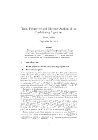
We observed (figure 1a) that we enumerate exponentially more elements
that expected if the target vector was too close to zero. In a second experiment
(figure 1b) we therefore increased the norm of x(1)
by a factor 2k
2

Level
|L
(i)
1 |+|L
(i)
2 |
2
1 156652
2 162259
3 173625
4 213778
5 406735
(a) n=50, R=1.09, α =1.12, short
target-vectors
Level
|L
(i)
1 |+|L
(i)
2 |
2
1 70068.5
2 79621.5
3 89920.5
4 103614
5 155649
(b) n=50, R=1.09, α =1.12, large
target-vectors
Figure 1: Comparison of list length for short and large target-vector
1.2 Test and experiment of parameters and environment
There are some parameters in the Dual-Sieving algorithm, namely the lattice
dimension, a factor to increase the sphere radius, the number of translated
lattices and the number of random bases for each lattice, as well as α and β.
Experiments were done with the following parameters:
• n ∈ {25, 35, 40, 45, 50, 60},
• factor to increase the sphere radius factorR ∈ {1.01, 1.02, 1.02, 1.04, 1.05, 1.06, 1.07, 1.08, 1.09, 1.1},
• number of translated lattices nbrep ∈ {1, 5},
• number of random bases per lattice nbessais ∈ {1, 3},
• the α parameter was set to its default value (α = 4
3 ) for all n, except
n ∈ {50, 60}.
Hardware used for experiments:
• Intel(R) Xeon(R) CPU, E5430 @ 2.66GHz
• 16 Gb RAM
3

2 Time analysis
Results of the time analysis are predictable: it is exponential in the dimension
and grows exponentially to the factorR. The interesting fact is that for n > 40,
algorithm works better with factorR = 1.07 than with factorR = 1.06 (Figure
2).
20.00 25.00 30.00 35.00 40.00 45.00
dimension
0.00
11.08
22.16
33.24
44.33
time(mimutes)
factorR=1.01 factorR=1.02 factorR=1.03 factorR=1.04 factorR=1.05 factorR=1.06
factorR=1.07 factorR=1.08
Time vs Dimension
Figure 2: Dimensions vs time (in minutes).
4

3 Merge steps
3.1 Average and variance of the list length
For low dimensions (n < 50) we used the asymmetric merge tree, α was fixed
to 4
3 , β was fixed to 3
2 . Results show that depending on the level the
average list length drops quickly. The reason for such loss of elements are the
two conditions: at the i-th step, new vectors should
• be in L (i−1)
• have a norm less than or equal to R(i−1)
These conditions are not satisfied for enough elements. To fix this, we can
decrease the value of the α parameter: the probability that a vector v will be
in both lattices is equal to 1
αn .
For high dimensions (n ∈ {50, 60}), we use α ∈ {1.11, 1.12} and factorR ∈
{1.01, 1.04, 1.05, 1.06, 1.07, 1.09}, symmetric merge tree and β fixed to 4
3 .
In the figure 3 and 4 you can see the average and the variance of a list length
per level for low dimensions using asymmetric merge tree and short target-
vectors.
0.00 1.00 2.00 3.00 4.00
Level
0.00
946.70
1893.41
2840.11
3786.82
factorR=01 factorR=02 factorR=03 factorR=04 factorR=05 factorR=06 factorR=07
factorR=08
List length average vs Level
n=35.
0.00 1.00 2.00 3.00 4.00
Level
0.00
3177.19
6354.39
9531.58
12708.77
factorR=08
n=40.
0.00 1.25 2.50 3.75 5.00
Level
0.00
11501.19
23002.38
34503.56
46004.75
factorR=08
n=45.
Figure 3: List length averages for low dimensions, asymmetric merge tree
0.00 1.00 2.00 3.00 4.00
Level
0.00
310.81
621.62
932.43
1243.24
factorR=08
List length variance vs Level
n=35.
0.00 1.00 2.00 3.00 4.00
Level
0.00
1223.55
2447.11
3670.66
4894.21
factorR=08
n=40.
0.00 1.25 2.50 3.75 5.00
Level
0.00
3226.39
6452.78
9679.17
12905.56
factorR=08
n=45.
Figure 4: List length variances for low dimensions, asymmetric merge tree
In the tables 5 you find the average list length per level for high dimensions
using symmetric merge tree. Note that for symmetric merge tree we have only
two branches with the same number of elements inside each pair of lists, so
5

this average was calculated as follows:
|L
(i)
1 |+|L
(i)
2 |
2 where |L
(i)
j | is the number of
elements inside of the list j on level i.
Level
|L
(i)
1 |+|L
(i)
2 |
2
1 1
2 179
3 3604.5
4 18927
5 78280
a) n=50, R=1.01, α =1.12, short
target-vectors
Level
|L
(i)
1 |+|L
(i)
2 |
2
1 2869
2 13600
3 33993.5
4 68635.5
5 179852
b) n=50, R=1.05, α =1.12, short
target-vectors
Level
|L
(i)
1 |+|L
(i)
2 |
2
1 156652
2 162259
3 173625
4 213778
5 406735
c) n=50, R=1.09, α =1.12, short
target-vectors
Level
|L
(i)
1 |+|L
(i)
2 |
2
1 2384024
2 2323117
3 2143358
4 1859734
5 1502343.5
6 1260579
7 1893701
e) n=60, R=1.09, α =1.12, short
target-vectors
Figure 5: List length averages for high dimensions, symmetric merge tree
6

3.2 Duplicates in list sorting
We have counted duplicates for low dimensions with an asymmetric merge tree.
The number of duplicates is not stable as the size of the lists does decrease.
On the ﬁgure 6 ans 7 you can see the average number and the variance of
number of duplicates by level for dimensions 35, 40, and 45.
0.00 1.00 2.00 3.00 4.00
Level
0.00
3713.58
7427.17
11140.75
14854.34
factorR=08
Duplicates average vs Level
n=35.
0.00 1.00 2.00 3.00 4.00
Level
0.00
17653.43
35306.87
52960.30
70613.73
factorR=08
n=40.
0.00 1.25 2.50 3.75 5.00
Level
0.00
83221.88
166443.75
249665.63
332887.51
factorR=08
n=45.
Figure 6: Duplicates averages
0.00 1.00 2.00 3.00 4.00
Level
0.00
62.59
125.19
187.78
250.38
factorR=08
Duplicates variance vs Level
n=35.
0.00 1.00 2.00 3.00 4.00
Level
0.00
116.03
232.06
348.08
464.11
factorR=08
n=40.
0.00 1.25 2.50 3.75 5.00
Level
0.00
304.94
609.87
914.81
1219.74
factorR=08
n=45.
Figure 7: Duplicates variances
7

4 Percentage of short vectors found
We are interested in the ratio of short vectors within all found vectors of C(0)
.
The short vector in this case is one of norm less than 1.1 ∗ |v|2 where v is a
known somehow short vector in L .
Results for low dimensions, using the asymmetric merge tree:
• n = 40, α = 4
3 , factorR = 1.06, rate= 1.45%
• n = 40, α = 4
3 , factorR = 1.07, rate= 1.45%
• n = 40, α = 4
3 , factorR = 1.08, rate= 0.7%
• n = 45, α = 4
3 , factorR = 1.07, rate= 0.57%
• n = 45, α = 4
3 , factorR = 1.08, rate= 0.2%
Results for high dimensions, using the symmetric merge tree:
• n = 50, α = 1.12, factorR = 1.06, rate= 0.7%, found vectors: 282, number
of short vectors: 2.
• n = 50, α = 1.12, factorR = 1.07, rate= 0.09%, found vectors: 13237,
number of short vectors: 12.
• n = 50, α = 1.12, factorR = 1.08, rate= 0.015%, found vectors: 95090,
number of short vectors: 14.
5 Conclusion
The number of experiments that we have done is not suﬃcient to make any
rigorous conclusion about the choice of parameters, targets or the eﬃciency of
the dual-sieve algorithm. Further experiments need to be performed for higher
dimensions, more random lattices and randomised bases.
However, the experiments gave rise to some improvements such as an in-
crease of the target vector norm which guarantees lists of average size. We also
compared the symmetric (single choice of target and having in lower levels) with
the asymmetric (new random targets in each level) merge tree. We saw that
a single random target vector reduces the memory considerably while keeping
enough randomness to lead solutions.
8

main

Recommended

Recommended

More Related Content

What's hot

What's hot (20)

Similar to main

Similar to main (20)

main