solution manual for heat conduction

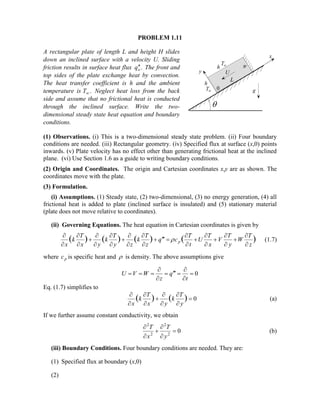
1. PROBLEM 1.11
A rectangular plate of length L and height H slides
down an inclined surface with a velocity U. Sliding
friction results in surface heat flux .
o
q 
 The front and
top sides of the plate exchange heat by convection.
The heat transfer coefficient is h and the ambient
temperature is .

T Neglect heat loss from the back
side and assume that no frictional heat is conducted
through the inclined surface. Write the two-
dimensional steady state heat equation and boundary
conditions.
(1) Observations. (i) This is a two-dimensional steady state problem. (ii) Four boundary
conditions are needed. (iii) Rectangular geometry. (iv) Specified flux at surface (x,0) points
inwards. (v) Plate velocity has no effect other than generating frictional heat at the inclined
plane. (vi) Use Section 1.6 as a guide to writing boundary conditions.
(2) Origin and Coordinates. The origin and Cartesian coordinates x,y are as shown. The
coordinates move with the plate.
(3) Formulation.
(i) Assumptions. (1) Steady state, (2) two-dimensional, (3) no energy generation, (4) all
frictional heat is added to plate (inclined surface is insulated) and (5) stationary material
(plate does not move relative to coordinates).
(ii) Governing Equations. The heat equation in Cartesian coordinates is given by
)
(
)
(
)
(
)
(
z
T
W
y
T
x
T
U
t
T
c
q
z
T
k
z
y
T
k
y
x
T
k
x
p






























V
 (1.7)
where p
c is specific heat and  is density. The above assumptions give
0













t
q
z
W
V
U
Eq. (1.7) simplifies to
0
)
(
)
( 









y
T
k
y
x
T
k
x
(a)
If we further assume constant conductivity, we obtain
0
2
2
2
2






y
T
x
T
(b)
(iii) Boundary Conditions. Four boundary conditions are needed. They are:
(1) Specified flux at boundary (x,0)
(2)

T
h
y
x
g
h 
T

U
0
W
L

2. PROBLEM 1.11 (continued)
o
q
y
x
T
k 





)
0
,
(
(2) Convection at surface ).
,
( W
x Pretending that heat flows in the positive y-direction,
conservation of energy, Fourier’s law of conduction and Newton’s law of cooling give
 





 T
W
x
T
h
y
W
x
T
k )
,
(
)
,
(
(3) Convection at surface (0,y). Pretending that heat flows in the positive x-direction,
conservation of energy, Fourier’s law of conduction and Newton’s law of cooling give
 
)
,
0
(
)
,
0
(
y
T
T
h
x
y
T
k 



 
(4) Insulated boundary at surface ).
,
( y
L Fourier’s law gives
0
)
,
(



x
y
L
T
(4) Checking. Dimensional check: Each term in boundary conditions (1), (2) and (3) has
units of flux.
Limiting check: Boundary conditions (2) and (3) should reduce to an insulated condition if h
= 0. Similarly, boundary condition (1) should describe an insulated surface if .
0



o
q Setting
h = 0 in conditions (2) and (3) and 0



o
q in (1) gives the description for an insulated
surface.
(5) Comments. (i) The four boundary conditions are valid for constant and variable
conductivity k. (ii) Formulating boundary conditions requires an understanding of what
takes place physically at the boundaries. (iii) Plate motion in this example should not be
confused with convection velocity appearing in the heat equation (1.7).

3. PROBLEM 2.17
A section of a long rotating shaft of radius o
r is buried in a
material of very low thermal conductivity. The length of the
buried section is L. Frictional heat generated in the buried
section can be modeled as surface heat flux. Along the buried
surface the radial heat flux is r
q 
 and the axial heat flux is .
x
q 

The exposed surface exchanges heat by convection with the
ambient. The heat transfer coefficient is h and the ambient
temperature is .

T Model the shaft as semi-infinite fin and
assume that all frictional heat is conducted through the shaft.
Determine the temperature distribution.
(1) Observations. (i) This is a constant area fin. (ii)
Temperature distribution can be assumed one dimensional. (iii)
The shaft has two sections. Surface conditions are different
for each of sections. Thus two equations are needed. (iv) Shaft
rotation generates surface flux in the buried section and does
not affect the fin equation.
(2) Origin and Coordinates. The origin is selected at one end of the fin and the coordinate
x is directed as shown.
(3) Formulation.
(i) Assumptions. (1) One-dimensional, (2) steady state, (3) constant cross-sectional area,
(4) uniform surface flux in the buried section, (5) ,
1

Bi (6) constant conductivity, (7) no
radiation (8) no energy generation and (9) uniform h and 
T .
(ii) Governing Equations. Since surface conditions are different for the two sections,
two fin equations are needed. Let
)
(
1 x
T = temperature distribution in the buried section, L
x 

0
)
(
2 x
T = temperature distribution in the exposed section, L
x
L 2


The heat equation for the buried section must be formulated using fin approximation.
Conservation of energy for the fin element dx gives
dx
dx
dq
q
dx
r
q
q x
x
o
r
x 



 
2 (a)
where x
q is the rate of heat conducted in the x-direction,
given by Fourier’s law
dx
dT
k
qx
1

 (b)
Substituting (b) into (a) and rearranging
0
2
2
1
2




o
r
kr
q
dx
T
d
, L
x 

0 (c)
The heat equation for constant area fin with surface convection is given by equation (2.9)
0
h

T

r
q
 x L
x
q 

dx
r
oq
r 


2
dx
dx
dq
q x
x 
x
q
dx

4. PROBLEM 2.17 (continued)
0
)
( 2
2
2
2


 
T
T
kA
hC
dx
T
d
c
, L
x  (d)
where C is the circumferance and c
A is the cross section area given by
o
r
C 
2
 (e)
2
o
r
A (f)
Using (c) and (d) to define m
o
c kr
h
kA
hC
m
2

 (g)
Subatituting (e) into (d)
0
)
( 2
2
2
2
2


 
T
T
m
dx
T
d
(h)
(iii) Boundary Conditions. Four boundary conditions are needed.
(1) Specified flux at x = 0
x
q
x
d
dT
k 



)
0
(
1
(i)
(2) Equality of temperature at x = L
)
(
)
( 2
1 L
T
L
T  (j)
(3) Equality of flux at x = L
x
d
L
dT
x
d
L
dT )
(
)
( 2
1
 (k)
(4) Finite temperature at 

x

)
(
2
T finite (l)
(4) Solution. The solutions to (c) is
1
1
2
1 )
( B
x
A
x
kr
q
x
T
o
r





 (m)
where 1
A and 1
B are constants of integration. The solution to (h) is given in Appendix A,
equation (A-2b)
mx
mx
e
B
e
A
T
x
T 
 

 2
2
2 )
( (n)
where 2
A and 2
B are constants of integration. Application of the four boundary conditions
gives the four constants
k
q
A x




1 (o)





 











 
k
q
L
kr
q
m
L
k
q
L
kr
q
T
B x
o
r
x
o
r
2
1
2
1 (p)

5. 2-1
PROBLEM 2.1
Radiation is used to heat a plate of thickness L and thermal
conductivity k. The radiation has the effect of volumetric energy
generation at a variable rate given by
bx
o e
q
x
q 






 )
(
where o
q 

 and b are constant and x is the distance along the
plate. The heated surface at x = 0 is maintained at uniform temperature o
T while the
opposite surface is insulated. Determine the temperature of the insulated surface.
(1) Observations. (i) This is a steady state one-dimensional problem. (ii) Use a rectangular
coordinate system. (iii) Energy generation is non-uniform. (iv) Two boundary conditions are
needed. The temperature is specified at one boundary. The second boundary is insulated. (v)
To determine the temperature of the insulated surface it is necessary to determine the
temperature distribution in the plate.
(2) Origin and Coordinates. A rectangular coordinate system is used with the origin at one
of the two surfaces. The coordinate x is oriented as shown.
(3) Formulation.
(i) Assumptions. (1) One-dimensional, (2) steady state, (3) stationary and (4) constant
properties.
(ii) Governing Equations. Introducing the above assumptions into eq. (1.8) gives
0
2
2





k
q
dx
T
d
(a)
where
k = thermal conductivity
q 

 = rate of energy generation per unit volume
T = temperature
x = independent variable
Energy generation q 

 varies with location according to
bx
o e
q
q 






 (b)
where o
q 

 and b are constant. Substituting (b) into (a) gives
0
2
2




 bx
o
e
k
q
dx
T
d
(c)
(iii) Boundary Conditions. Since (c) is second order with a single independent variable
x, two boundary conditions are needed.
(1) Specified temperature at x = 0
T(0) = o
T (d)
(2) The surface at x = L is insulated
L
radiation
0
)
(x
q


x
o
T

6. 2-2
PROBLEM 2.1 (continued)
0
)
(

x
d
L
dT
(e)
(4) Solution. Separating variables and integrating (c) twice
2
1
2
)
( C
x
C
e
k
b
q
x
T bx
o






 
(f)
where C1 and C2 are constants of integration. Application of boundary conditions (d) and
(e) gives C1 and C2
,
1
bL
o
e
bk
q
C 





k
b
q
T
C o
o 2
2




 (g)
Substituting (g) into (f)
  o
bL
bx
o
T
bxe
e
k
b
q
x
T 





 

1
)
( 2
(h)
The temperature of the insulated surface is obtained by setting x = L in (h)
  o
bL
o
T
e
bL
k
b
q
L
T 





 
)
1
(
1
)
( 2
(i)
Expressing (h) and (i) in dimensionless form gives
bL
L
x
bL
o
o
e
L
x
bL
e
k
b
q
T
x
T 








)
/
)(
(
1
)
( )
/
(
2
(j)
and
bL
o
o
e
bL
k
b
q
T
L
T 







)
1
(
1
)
(
2
(k)
(5) Checking. Dimensional check: Each term in solution (h) has units of temperature.
Boundary conditions check: Setting x = 0 in (h) gives T(0) = o
T . Thus boundary condition
(d) is satisfied. To check condition (e) solution (h) is differentiated to obtain
 
bL
bx
o
be
be
k
b
q
x
d
dT 





 2
(m)
Evaluation (m) at x = L shows that condition (e) is satisfied.
Differential equation check: Direct substitution of (h) into equation (c) shows that the
solution satisfies the governing equation.
Global energy conservation check: The total energy generated in the plate, g
E
 , must be
equal to the energy conducted from the plate at x = 0. Energy generated is given by
)
1
(
)
(
0
0
bL
o
L
bx
o
L
g e
b
q
dx
e
q
dx
x
q
E 













 

 (k)
Energy conducted at x = 0, )
0
(
E
 , is determined by substituting (m) into Fourier’s law

7. 2-3
PROBLEM 2.1 (continued)
)
1
(
)
0
(
)
0
( bL
o
e
b
q
x
d
dT
k
E 








 (l)
The minus sign indicates that heat is conducted in the negative x-direction. Thus energy is
conserved.
Limiting check: For the special case of ,
0




q temperature distribution should be uniform
given by .
)
( o
T
x
T  Setting 0




o
q in (h) gives the anticipated result.
(6) Comments. (i) The solution to the special case of constant energy generation
corresponds to .
0

b However, setting 0

b in solution (h) gives 0/0. To obtain the
solution to this case it is necessary to set 0

b in differential equation (c) and solve the
resulting equation. (ii) The dimensionless solution is characterized by a single dimensionless
parameter bL.

8. 2-4
PROBLEM 2.2
Repeat Example 2.3 with the outer plates generating energy at a rate q 

 and no energy is
generated in the inner plate.
(1) Observations. (i) The three plates form a composite wall. (ii) The geometry can be
described by a rectangular coordinate system. (iii) Due to symmetry, no heat is conducted
through the center plate. Thus the center plate is at a uniform temperature. (iv) Heat
conduction is assumed to be in the direction normal to the three plates. (v) This problem
reduces to a single heat generating plate in which one side is maintained at a specified
temperature and the other side is insulated.
(2) Origin and Coordinates. Since only one plate needs to be analyzed, the origin and
coordinate x are selected as shown.
(3) Formulation.
(i) Assumptions. (1) One-dimensional, (2) steady state and (3) constant conductivity of
the heat generating plate.
(ii) Governing Equations. Let the subscript 2 refer to the heat generating plate. Based
on the above assumptions, )
8
.
1
(
.
eq gives
0
2
2
2
2





k
q
dx
T
d
(a)
where
2
k = thermal conductivity
q 

 = rate of energy generation per unit volume
T = temperature
x = coordinate
(iii) Boundary Conditions. Since (a) is second order with a single independent variable
x, two boundary conditions are needed.
(1) Specified temperature at x = 0
o
T
T 
)
0
(
2 (b)
(2) Insulated surface at 2
L
x 
0
)
( 2
2

x
d
L
dT
(c)
where 2
L is the thickness of the heat generating plate.
(4) Solution. Integrating (a) twice gives
2
1
2
2
2
2
)
( C
x
C
x
k
q
x
T 





 (d)
where 1
C and 2
C are constants of integration. Application of boundary conditions (b) and
(c) gives 1
C and 2
C
q 


2
L
2
L
1
L
2
k
o
T
o
T
0
x 1
k
2
k
q 


q 

 2
k

9. 2-5
PROBLEM 2.2 (continued)
2
2
1
k
L
q
C



 , o
T
C 
2 (e)
Substituting (e) into (d) gives the temperature distribution in the heat generating plate
  o
T
x
L
k
x
q
x
T 




 1
)
/
2
(
2
)
( 2
2
2
2 (f)
To determine the temperature distribution in the center plate we apply continuity of
temperature at 2
L
x 
)
(
)
( 2
2
2
1 L
T
L
T  (g)
Noting that the center plate must be at a uniform temperature, evaluating (f) at 2
L
x  and
substituting into (g) gives
o
T
k
L
q
L
T
L
T
x
T 






2
2
2
2
2
2
1
1
2
)
(
)
(
)
( (h)
Expressing (f) and (h) in dimensionless form gives
 
)
/
(
2
2
1
)
(
2
2
2
2
2
2
L
x
L
x
k
L
q
T
x
T o






(i)
and
2
1
)
(
2
2
2
2





k
L
q
T
x
T o
(j)
(5) Checking. Dimensional check: Each term in (f) has units of temperature.
Boundary conditions check: Substitution of solutions (f) into (b) and (c) shows that the two
boundary conditions are satisfied.
Differential equation check: Direct substitution of (f) into equation (a) shows that the
solution satisfies the governing equation.
Global energy conservation check: The total energy generated in the plate, g
E
 , must be
equal to the energy conducted from the plate at x = 0. Energy generated is given by
2
AL
q
Eg 



 (k)
where A is surface area. Energy conducted at x = 0, )
0
(
E
 , is determined by differentiation
(f) and substituting into Fourier’s law
2
2
2
)
0
(
)
0
( AL
q
x
d
dT
A
k
E 






 (m)
The minus sign indicates that heat is conducted in the negative x-direction. Equations (k)
and (m) show that energy is conserved.

10. 2-6
PROBLEM 2.2 (continued)
Limiting check: If energy generation vanishes, the composite wall should be at a uniform
temperature .
o
T Setting 0




q in (f) and (h) gives .
)
(
)
( 2
1 o
T
x
T
x
T 

(6) Comments. (i) An alternate approach to solving this problem is to consider half the
center plate and the heat generating plate as a composite wall, note symmetry, write two
differential equations and four boundary conditions and solve for )
(
1 x
T and ).
(
2 x
T Clearly
this is a longer approach to solving the problem. (ii) No parameter characterizes the solution.

11. 2-7
PROBLEM 2.3
A plate of thickness 1
L and conductivity 1
k moves with a
velocity U over a stationary plate of thickness 2
L and
conductivity .
2
k The pressure between the two plates is P
and the coefficient of friction is .
 The surface of the
stationary plate is insulated while that of the moving plate is
maintained at constant temperature .
o
T Determine the steady
state temperature distribution in the two plates.
(1) Observations. (i) The two plates form a composite wall. (ii) The geometry can be
described by a rectangular coordinate system. (iii) Heat conduction is assumed to be in the
direction normal to the two plates. (iv) Since the stationary plate is insulated no heat is
conducted through it. Thus it is at a uniform temperature. (v) All energy dissipated due to
friction at the interface is conducted through the moving plate. (vi) This problem reduces to
one-dimensional steady state conduction in a single plate with specified flux at one surface
and a specified temperature at the opposite surface. (vii) Plate motion plays no role in the
governing equation since no heat is conducted in the direction of motion.
(2) Origin and Coordinates. Since only one plate needs to be analyzed, the origin is
selected at the interface and the coordinate x is directed as shown.
(3) Formulation.
(i) Assumptions. (1) One-dimensional, (2) steady state, (3) constant conductivity of the
moving plate, (4) no energy generation and (5) uniform energy dissipation at the interface.
(ii) Governing Equations. Let the subscript 1 refer to the moving plate. Based on the
above assumptions, )
8
.
1
(
.
eq applied to the moving plate gives
0
2
1
2

dx
T
d
(a)
(iii) Boundary Conditions. Since (a) is second order with a single independent variable
x, two boundary conditions are needed.
(1) Specified heat flux at x = 0 . Fourier’s law gives
PU
x
d
dT
k 


)
0
(
1
1 (b)
where
1
k = thermal conductivity
P = interface pressure
U = plate velocity
 = coefficient of friction
(2) Specified temperature at 1
L
x 
o
T
L
T 
)
( 1
1 (c)
where 1
L is the thickness of the moving plate.
2
k
1
k
2
L
1
L
U
o
T
x
0

12. 2-8
PROBLEM 2.3 (continued)
(4) Solution. Integrating (a) twice gives
2
1
1 )
( C
x
C
x
T 
 (d)
where 1
C and 2
C are constants of integration. Application of boundary conditions (b) and
(c) gives 1
C and 2
C
1
1
k
PU
C


 , 1
1
2 L
k
PU
T
C o


 (e)
Substituting (e) into (d) gives the temperature distribution in the moving plate
  o
T
L
x
k
PUL
x
T 

 )
/
(
1
)
( 1
1
1
1

(f)
To determine the temperature distribution in the stationary plate we apply continuity of
temperature at x = 0
)
0
(
)
0
( 1
2 T
T  (g)
Noting that the stationary plate must be at a uniform temperature, evaluating (f) at x = 0 and
substituting into (g) gives
o
T
k
PUL
T
T
x
T 



1
1
1
2
2 )
0
(
)
0
(
)
(

(h)
Expressing (f) and (h) in dimensionless form gives
1
1
1
1
1
)
(
L
x
k
PUL
T
x
T o




(i)
1
)
(
1
1
1


k
PUL
T
x
T o

(j)
(5) Checking. Dimensional check: Each term in (f) has units of temperature
Boundary conditions check: Substitution of solutions (f) into (b) and (c) shows that the two
boundary conditions are satisfied.
Differential equation check: Direct substitution of (f) into equation (a) shows that the
solution satisfies the governing equation.
Limiting check: If no energy is added at the interface ( 0

 or U = 0 or P = 0), the two
plates should be at a uniform temperature .
o
T Setting any of the quantities  , U or P equal
to zero in (f) and (h) gives .
)
(
)
( 2
1 o
T
x
T
x
T 

(6) Comments. (i) An alternate approach to solving this problem is to consider the two
plates as a composite wall, write two differential equations and four boundary conditions
and solve for )
(
1 x
T and ).
(
2 x
T Clearly this is a longer approach to solving the problem. (ii)
No parameter characterizes the solution.

13. 2-9
PROBLEM 2.4
A thin electric element is wedged between two plates of
conductivities 1
k and 2
k . The element dissipates uniform
heat flux o
q 
 . The thickness of one plate is 1
L and that of
the other is 2
L . One plate is insulated while the other
exchanges heat by convection. The ambient temperature is

T and the heat transfer coefficient is h. Determine the
temperature of the insulated surface for one-dimensional
steady state conduction.
(1) Observations. (i) The two plates form a composite wall. (ii) The geometry can be
described by a rectangular coordinate system. (iii) Heat conduction is assumed to be in the
direction normal to the two plates. (iv) Since no heat is conducted through the insulated
plate, its temperature is uniform equal to the interface temperature. (v) All energy dissipated
by the element at the interface is conducted through the upper plate. (vi) This problem
reduces to one-dimensional steady state conduction in a single plate with specified flux at
one surface and convection at the opposite surface. (vii) To determine the temperature of the
insulated surface it is necessary to determine the temperature distribution in the upper plate.
(2) Origin and Coordinates. Since only one plate needs to be analyzed, the origin is
selected at the interface and coordinate x is directed as shown.
(3) Formulation.
(i) Assumptions. (1) One-dimensional, (2) steady state, (3) constant conductivity of the
upper plate, (4) no energy generation and (5) uniform energy dissipation at the interface.
(ii) Governing Equations. Let the subscript 1 refer to the upper plate. Based on the
above assumptions, )
8
.
1
(
.
eq applied to the upper plate gives
0
2
1
2

dx
T
d
(a)
(iii) Boundary Conditions. Since (a) is second order with a single independent variable
x, two boundary conditions are needed.
(1) Specified heat flux at x = 0
o
q
x
d
dT
k 



)
0
(
1
1 (b)
(2) Convection at 1
L
x  . Fourier’s law and Newton’s law of cooling give
 



 T
L
T
h
x
d
L
dT
k )
(
)
(
1
1
1
1
1 (c)
where 1
L is the thickness of the upper plate.
(4) Solution. Integrating (a) twice gives
2
1
1 )
( C
x
C
x
T 
 (d)
-
+
1
k
2
k
1
L
2
L

T
h
,
0
x

14. 2-10
PROBLEM 2.4 (continued)
where 1
C and 2
C are constants of integration. Application of boundary conditions (b) and
(c) gives 1
C and 2
C
1
1
k
q
C o



 ,   




 T
k
hL
h
q
C o
1
)
/
( 1
1
2 (e)
Substituting (e) into (d) and rearranging gives the temperature distribution in the upper plate












 T
L
x
k
hL
h
q
x
T o
1
1
)
( )
(
1
1
1
1 (f)
To determine the temperature distribution in the insulated plate we apply continuity of
temperature at x = 0
)
0
(
)
0
( 1
2 T
T  (g)
Noting that the stationary lower plate must be at a uniform temperature, evaluating (f) at x =
0 and substituting into (g) gives













 T
k
hL
h
q
T
T
x
T o
1
)
0
(
)
0
(
)
(
1
1
1
2
2 (h)
Equation (h) gives the temperature of the insulated surface.
Expressing (f) and (h) in dimensionless form gives
1
1
)
(
)
(
1
1





 
L
x
Bi
h
q
T
x
T
o
(i)
and
Bi
h
q
T
x
T
o




 
1
)
(
1
(j)
where Bi is the Biot number defined as
1
1
k
hL
Bi  (k)
(5) Checking. Dimensional check: Each term in (f) has units of temperature.
Boundary conditions check: Substitution of solution (f) into (b) and (c) shows that the two
boundary conditions are satisfied.
Differential equation check: Direct substitution of (f) into equation (a) shows that the
solution satisfies the governing equation.
Limiting check: (i) If no energy is added at the interface, the two plates should be at a
uniform temperature .

T Setting 0



o
q in (f) and (h) gives .
)
(
)
( 2
1 

 T
x
T
x
T (ii) If h = 0,

15. 2-11
PROBLEM 2.4 (continued)
no heat can leave the plates and thus their temperature will be infinite. Setting h = 0 in (f)
and (h) gives .
)
(
)
( 2
1 

 x
T
x
T
Qualitative check: Increasing interface energy input increases the temperature level in the
two plates. Equations (f) and (h) exhibit this behavior.
(6) Comments. (i) An alternate approach to solving this problem is to consider the two
plates as a composite wall, write two differential equations and four boundary conditions
and solve for )
(
1 x
T and ).
(
2 x
T Clearly this is a longer approach to solving the problem. (ii)
The problem is characterized by a single dimensionless parameter 1
1 / k
hL which is the Biot
number. This parameter appears in problems involving surface convection.

16. 2-12
PROBLEM 2.5
A thin electric element is sandwiched between two plates of
conductivity k and thickness L each. The element dissipates a
flux .
o
q 
 Each plate generates energy at a volumetric rate
of q 

 and exchanges heat by convection with an ambient fluid
at .

T The heat transfer coefficient is h. Determine the temperature
of the electric element.
(1) Observations. (i) The two plates form a composite wall. (ii) The geometry can be
described by a rectangular coordinate system. (iii) Heat conduction is assumed to be in the
direction normal to the two plates. (iv) Symmetry requires that half the energy dissipated by
the element at the interface is conducted through the upper plate and the other half is
conducted through the lower plate. Thus only one plate needs to be analyzed.(v) The
problem reduces to one-dimensional steady state conduction in a single plate with energy
generation having specified flux at one surface and convection at the opposite surface. (vi)
To determine the temperature of the element it is necessary to determine the temperature
distribution in one of the two plates.
(2) Origin and Coordinates. The upper plate is considered for analysis. The origin is
selected at the upper surface and coordinate x is directed as shown.
(3) Formulation.
(i) Assumptions. (1) One-dimensional, (2) steady state, (3)
constant conductivity of the upper plate, (4) uniform energy
generation and (5) uniform energy dissipation at the interface.
(ii) Governing Equations. Let the subscript 1 refer to the
upper plate. Based on the above assumptions, )
8
.
1
(
.
eq applied to
the upper plate gives
0
2
1
2





k
q
dx
T
d
(a)
(iii) Boundary Conditions. Since (a) is second order with a single independent variable
x, two boundary conditions are needed.
(2) Specified heat flux at x = L
2
)
(
1 o
q
x
d
L
dT
k




 (b)
(2) Convection at 0

x . Fourier’s law and Newton’s law of cooling give
 
)
0
(
)
0
(
1
1
T
T
h
x
d
dT
k 

  (c)
where L is the thickness of the upper plate.
(4) Solution. Integrating (a) twice gives
2
1
2
1
2
)
( C
x
C
x
k
q
x
T 





 (d)
+ _
0
x
L
L
q


q



T
h,

T
h,
+ _
0
x
L q



T
h
,
2
o
q


17. 2-13
PROBLEM 2.5 (continued)
where 1
C and 2
C are constants of integration. Application of boundary conditions (b) and
(c) gives 1
C and 2
C
k
L
q
k
q
C o 






2
1 ,
h
L
q
h
q
T
C o 






 
2
2 (e)
Substituting (e) into (d) and rearranging gives the temperature distribution in the upper plate
2
1
2
2
2
)
( x
k
q
x
k
L
q
k
q
h
L
q
h
q
T
x
T o
o 








 













  (f)
Expressing (f) in dimensionless form gives
2
1
2
1
2
1
/
)
(






























 
L
x
Bi
L
x
Bi
L
q
q
h
L
q
T
x
T o
(g)
where Bi is the Biot number defined as
k
hL
Bi  (h)
To determine the temperature of the electric element set x = L in (g)
  1
2
1
2
/
)
(
1












  Bi
Bi
L
q
q
h
L
q
T
L
T o
(i)
(5) Checking. Dimensional check: Each term in (g) is dimensionless.
Boundary conditions check: Substitution of solution (f) into (b) and (c) shows that the two
boundary conditions are satisfied.
Differential equation check: Direct substitution of (f) into equation (a) shows that the
solution satisfies the governing equation.
Limiting check: (i) If no energy is added at the interface and there is no energy generation
the two plates should be at a uniform temperature .

T Setting 0






 q
qo in (f) gives
.
)
(
1 
 T
x
T (ii) If h = 0, no heat can leave the plate and thus the temperature will be infinite.
Setting h = 0 in (f) gives .
)
(
1 

x
T
Qualitative check: Increasing interface energy input and/or energy generation increases the
temperature level in the plate. Equation (f) exhibit this behavior.
(6) Comments. (i) An alternate approach to solving this problem is to consider the two
plates as a composite wall, write two differential equations and four boundary conditions
and solve for )
(
1 x
T and ).
(
2 x
T Clearly this is a longer approach to solving the problem. (ii)
The solution is characterized by two parameters: the convection parameter Bi and the ratio of
energy dissipated in the element to energy generation, .
/ L
q
qo 





18. 2-14
PROBLEM 2.6
One side of a plate is heated with uniform flux o
q 
 while the other side exchanges heat by
convection and radiation. Surface emissivity is ,
 heat transfer coefficient h, ambient
temperature ,

T surroundings temperature ,
sur
T plate thickness L and the conductivity is k.
Assume one-dimensional steady state conduction and use a simplified radiation model.
Determine:
[a] The temperature distribution in the plate.
[b] The two surface temperatures for:
h = 27 C
W/m o
2
 , k = 15 C
W/m o
 , L = 8 cm,  = 0.95,
o
q 
 =19,500 2
W/m , sur
T = 18 C
o
, 
T = 22 C
o
.
(1) Observations. (i) This is a one-dimensional steady state problem. (ii) Two boundary
conditions are needed. (iii) Cartesian geometry. (iv) Specified flux at one surface and
convection and radiation at the opposite surface. (v) Since radiation is involved in this
problem, temperature units should be expressed in kelvin
(2) Origin and Coordinates. The origin and coordinate x are shown.
(3) Formulation.
(i) Assumptions. (1) Steady state, (2) one-dimensional, (3) constant properties, (4) no
energy generation, (5) small gray surface which is enclosed by a much larger surface, (6)
uniform conditions at the two surfaces and (7) stationary material.
(ii) Governing Equations. Based on the above assumptions, the heat equation in
Cartesian coordinates is given by
0
2
2

dx
T
d
(a)
(iii) Boundary Conditions. Two boundary conditions are needed. They are:
(1) Specified flux at 0

x
o
q
x
d
T
d
k 



)
0
(
(b)
where

k thermal conductivity = 15 C
W/m o




o
q surface flux = 19,500 2
W/m
(2) Convection and radiation at L
x  . Conservation of energy, Fourier’s law of
conduction, Newton’s law of cooling and Stefan-Boltzmann radiation law give
   
4
4
)
(
)
(
)
(
sur
T
L
T
T
L
T
h
x
d
L
dT
k 



  
 (c)
where

h heat transfer coefficient = 27 C
W/m o
2
 = 27 K
W/m2

0

T
h,
x
o
q

sur
T
k
L

19. 2-15
PROBLEM 2.6 (continued)

L plate thickness = 8 cm

T = ambient temperature = 22 C
o
= (22 + 273.15) K = 295.15 K
sur
T = surroundings temperature = 18 C
o
= (18 + 273.15) K = 291.15 K

 emissivity = 0.95

 Stefan-Boltzmann constant = 8
10
67
.
5 
 4
2
K
W/m 
(4) Solution. Integrating (a) twice gives
2
1
)
( C
x
C
x
T 
 (d)
where 1
C and 2
C are constants of integration. Application of boundary conditions (b) and
(c) gives
k
q
C o




1 (e)

























 
4
4
2
2 )
( sur
o
o
o T
C
L
k
q
T
C
L
k
q
h
q 
 (f)
Equation (f) gives the constant 2
C . However, this equation must be solved for 2
C by trial
and error.
(5) Checking. Dimensional Check: Each term in equations (b), (c) and (f) has units of flux.
Differential equation check: Solution (d) satisfies the governing equation (a).
(6) Computations. Equation (e) gives
m
K
1300
m
C
1300
C)
W/m-
(
15
)
(W/m
19,500
C
o
o
2
1 





Equation (f) gives




























)
K
(
)
15
.
291
(
m)
(
08
.
0
K)
-
W/m
(
15
)
(W/m
19,500
-
)
K
-
W/m
(
10
67
.
5
)
95
.
0
(
K)
(
15
.
295
m)
(
08
.
0
K)
-
W/m
(
15
)
(W/m
19,500
-
K)
-
W/m
(
7
2
)
(W/m
19,500
4
4
4
2
2
4
2
8
2
2
2
2
C
C
Solving this equation for 2
C by trial and error gives
K
9
.
761
C2 
Substituting 1
C and 2
C into (d) gives
x
x
T )
K/m
(
1300
)
K
(
9
.
761
)
( 
 (g)
Surface temperatures at x = 0 and x = L are determined using (g)

20. 2-16
PROBLEM 2.6 (continued)
9
.
761
)
0
( 
T K
9
.
657
)
( 
L
T K
(7) Comments. (i) A trial and error procedure was required to solve this problem. (ii) Care
should be exercised in selecting the correct units for temperature in radiation problems. (iii)
With the two temperatures determined a numerical check based on conservation of energy
can be made.
Energy flux entering plate = Energy flux conducted through the plate = Energy flux leaving (h)
Energy flux entering plate = 500
,
19



o
q 2
W/m
Energy flux conducted through the plate =
k
L
L
T
T
/
)
(
)
0
( 
Energy flux leaving 






















 
4
4
2
2 )
( sur
o
o
T
C
L
k
q
T
C
L
k
q
h 

Numerical computations show that each term in (h) is equal to 19,500 2
W/m .

21. 2-17
PROBLEM 2.7
A hollow shaft of outer radius s
R and inner radius i
R rotates
inside a sleeve of inner radius s
R and outer radius .
o
R Frictional
heat is generated at the interface at a flux .
s
q 
 At the inner shaft
surface heat is added at a flux .
i
q 
 The sleeve is cooled by
convection with a heat transfer coefficient h. The ambient
temperature is .

T Determine the steady state one-dimensional
temperature distribution in the sleeve.
(1) Observations. (i) The shaft and sleeve form a composite
cylinder. (ii) Use a cylindrical coordinate system. (iii) Heat conduction is assumed to be in
the radial direction only. (iv) At steady state, energy entering the shaft at i
R must be equal
to energy leaving at o
R . (v) Frictional energy dissipated at the interface and energy added at
i
R must be conducted through the sleeve. (vi) This problem reduces to one-dimensional
steady state conduction in a hollow cylinder (sleeve) with specified flux at the inside surface
and convection at the outside surface.
(2) Origin and Coordinates. The origin is selected at the center and the coordinate r is
directed as shown.
(3) Formulation.
(i) Assumptions. (1) One-dimensional, (2) steady state, (3) constant conductivity of the
sleeve, (4) no energy generation, and (5) uniform frictional energy at the interface.
(ii) Governing Equations. Based on the above assumptions, )
11
.
1
(
.
eq applied to the sleeve
gives
0
)
( 
dr
dT
r
dr
d
(a)
(iii) Boundary Conditions. Since (a) is second order with a single independent variable
r, two boundary conditions are needed.
(1) Specified heat flux at s
R
r  . Fourier’s law gives
sl
s
q
dr
R
dT
k 



)
(
(b)
where sl
q 
 is the heat flux added to the sleeve at .
s
R
r  This flux is the sum of frictional
energy generated at the interface and energy added at i
R . That is
o
s
sl q
q
q 






 (c)
where
o
q 
 = heat flux leaving the shaft at s
R
s
q 
 = heat flux generated by friction at the interface s
R
sl
q 
 = total heat flux entering the sleeve at s
R
At steady state, conservation of energy applied to the shaft requires that energy entering the
shaft at i
R be equal to energy leaving it at .
s
R Thus
shaft
sleeve
o
R s
R

T
h,
s
q 

i
q 

i
R

22. 2-18
PROBLEM 2.7 (continued)
o
s
i
i q
R
q
R 



 
 2
2
Or
i
s
i
o q
R
R
q 



 (d)
Substituting (c) and (d) into (b) gives the boundary condition at s
R
i
s
i
s
s
q
R
R
q
dr
R
dT
k 






)
(
(e)
(2) Convection at o
R
r  . Fourier’s law and Newton’s law of cooling give
 



 T
R
T
h
r
d
R
dT
k o
o
)
(
)
(
(f)
(4) Solution. Integrating (a) twice gives
2
1 ln
)
( C
r
C
r
T 
 (g)
where 1
C and 2
C are constants of integration. Application of boundary conditions (e) and (f)
gives 1
C and 2
C
 
i
s
i
s
s
q
R
R
q
k
R
C 





 )
/
(
1 ,   
o
o
i
s
i
s
s
R
hR
k
q
R
R
q
k
R
T
C ln
)
/
(
)
/
(
2 






  (h)
Substituting (h) into (g) and rearranging gives the temperature distribution in the sleeve
   







 T
hR
k
r
R
q
R
R
q
k
R
r
T o
o
i
s
i
s
s
)
/
(
)
/
ln(
)
/
(
)
( (i)
Expressing (i) in dimensionless form gives
 
)
/
1
(
)
/
ln(
1
)
(
Bi
r
R
R
q
R
q
k
R
q
T
r
T
o
s
i
i
s
s















 
(j)
where the Biot number Bi is defined as
k
hR
Bi o
 (k)
(5) Checking. Dimensional check: Each term in (i) has units of temperature. Each term in (j)
is dimensionless.
Boundary conditions check: Substitution of solutions (i) into (e) and (f) shows that the two
boundary conditions are satisfied.
Differential equation check: Direct substitution of (i) into (a) shows that the solution
satisfies the governing equation.
Limiting check: (i) If no energy is added to the shaft at i
R and no frictional heat is generated
at the interface s
R , the sleeve should be at a uniform temperature .

T Setting 0





 s
i q
q in

23. 2-19
PROBLEM 2.7 (continued)
(i) gives .
)
( 
 T
r
T (ii) If h = 0, no heat can leave the sleeve and the temperature will be
infinite. Setting h = 0 in (i) gives .
)
( 

r
T
(6) Comments. (i) An alternate approach to solving this problem is to consider the shaft and
sleeve as a composite cylinder, write two differential equations and four boundary
conditions and solve for the temperature distribution in both shaft and cylinder. Clearly this
is a longer approach to solving the problem. (ii) Two parameters characterize the solution:
The Biot number and heat ratio )
/
( s
s
i
i R
q
R
q 


 .

24. 2-20
PROBLEM 2.8
A hollow cylinder of inner radius i
r and outer radius o
r is heated
with flux i
q 
 at its inner surface. The outside surface exchanges
heat with the ambient and surroundings by convection and
radiation. The heat transfer coefficient is h, ambient temperature
,

T surroundings temperature sur
T and surface emissivity is .

Assume steady state one-dimensional conduction and use a
simplified radiation model. Determine:
[a] The temperature distribution in the cylinder.
[b] The inner and outer surface temperatures for:
i
q 
 = 35,500 2
W/m , 
T = 24 C
o
, sur
T = 14 C
o
, k = 3.8 C
W/m o
 , o
r = 12 cm,
i
r = 5.5 cm, h = 31.4 C
W/m o
2
 ,  = 0.92
(1) Observations. (i) This is a one-dimensional steady state problem. (ii) Two boundary
conditions are needed. (iii) Cylindrical geometry. (iv) Specified flux at the inner surface and
convection and radiation at the outer surface. (v) Since radiation is involved in this problem,
temperature units should be expressed in kelvin
(2) Origin and Coordinates. The origin and coordinate r are shown.
(3) Formulation.
(i) Assumptions. (1) Steady state, (2) one-dimensional, (3) constant properties, (4) no
energy generation, (5) small gray surface which is enclosed by a much larger surface, (6)
uniform conditions at the two surfaces and (7) stationary material.
(ii) Governing Equations. Based on the above assumptions, the heat equation in
Cartesian coordinates is given by
0
)
( 
dr
dT
r
dr
d
(a)
(iii) Boundary Conditions. Two boundary conditions are needed. They are:
(2) Specified flux at i
r
r 
i
i
q
r
d
r
T
d
k 



)
(
(b)
where

k thermal conductivity = 3.8 C
W/m o




o
q surface flux = 35,500 2
W/m

i
r inside radius = 5.5 cm
(2) Convection and radiation at o
r
r  . Conservation of energy, Fourier’s law of
conduction, Newton’s law of cooling and Stefan-Boltzmann radiation law give
   
4
4
)
(
)
(
)
(
sur
o
o
o
T
r
T
T
r
T
h
r
d
r
dT
k 



  
 (c)

T
h, 
i
q 

sur
T
o
r
i
r
r

25. 2-21
PROBLEM 2.8 (continued)
where

h heat transfer coefficient = 31.4 C
W/m o
2
 = 27 K
W/m2


o
r outside radius = 12 cm

T = ambient temperature = 24 C
o
= (24 + 273.15) K = 297.15 K
sur
T = surroundings temperature = 14 C
o
= (14 + 273.15) K = 287.15 K

 emissivity = 0.92

 Stefan-Boltzmann constant = 8
10
67
.
5 
 4
2
K
W/m 
(4) Solution. Integrating (a) twice gives
2
1 ln
)
( C
r
C
r
T 
 (d)
where 1
C and 2
C are constants of integration. Application of boundary conditions (b) and
(c) gives
i
i
r
k
q
C




1 (e)

























 
4
4
2
2 )
( ln
ln sur
o
i
i
o
i
i
i
o
i
T
C
r
r
k
q
T
C
r
r
k
q
h
q
r
r

 (f)
Equation (f) gives the constant 2
C . However, this equation must be solved for 2
C by trial
and error.
(5) Checking. Dimensional Check: Each term in equations (b), (c) and (f) has units of flux.
Differential equation check: Solution (d) satisfies the governing equation (a).
(6) Computations. Equation (e) gives
m
K
82
.
513
m
C
82
.
513
m)
(
055
.
0
C)
W/m-
(
8
.
3
)
(W/m
35,500
C
o
o
2
1 





Equation (f) gives




























)
K
(
)
15
.
287
(
m)
(
12
.
0
ln
)
(W/m
35,500
K)
-
W/m
(
8
.
3
0.055(m)
-
)
K
-
W/m
(
10
67
.
5
)
92
.
0
(
K)
(
15
.
297
.
m)
(
12
.
0
ln
)
(W/(W/m
500
,
35
K)
-
W/m
(
8
.
3
m)
(
055
.
0
-
K)
-
W/m
(
4
.
31
)
(W/m
35,500
0.12(m)
0.055(m)
4
4
4
2
2
4
2
8
2
2
2
2
C
C
Solving this equation for 2
C by trial and error gives
K
8
.
484
C2 

Substituting (e) and 2
C into (d) gives
r
r
k
q
r
T i
i
ln
)
K
(
8
.
484
)
( 

 (g)

26. 2-22
PROBLEM 2.8 (continued)
To determine the inside surface temperature set i
r
r  in (g)
K
48
.
1005
)
m
(
055
.
0
ln
)
m
(
055
.
0
)
C
m
/
W
(
8
.
3
)
C
m
/
W
(
500
,
35
)
K
(
8
.
484
)
( o
o
2






i
r
T
Similarly, the outside surface temperature is
K
625
.
604
)
m
(
055
.
0
ln
)
m
(
055
.
0
)
C
m
/
W
(
8
.
3
)
C
m
/
W
(
500
,
35
)
K
(
8
.
484
)
( o
o
2






o
r
T
(7) Comments. (i) A trial and error procedure was required to solve this problem. (ii) Care
should be exercised in selecting the correct units for temperature in radiation problems. (iii)
With the two temperatures determined a numerical check based on conservation of energy
for a tube of length L can be made:
Energy entering tube at i
r = Energy conducted through tube = Energy leaving tube at o
r (h)
Energy entering tube = i
i q
r
L
q


 
2 W/m
Energy conducted through tube =
i
o
o
i
r
r
k
r
T
r
T
L
q
ln
2
1
)
(
)
(



Energy flux leaving at
L
q
ro     
4
4
)
(
2
)
(
2 sur
o
o
o
o T
r
T
r
T
r
T
h
r 


  



Numerical computations show that each term in (h) is equal to 12267.9 W/m.

27. 2-23
PROBLEM 2.9
Radiation is used to heat a hollow sphere of inner radius ,
i
r outer radius o
r and
conductivity k. Due to the thermal absorption characteristics of the material the radiation
results in a variable energy generation rate given by
2
2
)
(
o
o
r
r
q
r
q 






where o
q 

 is constant and r is the radial coordinate. The
inside surface is insulated and the outside surface is
maintained at temperature .
o
T Assume steady state one-
dimensional conduction, determine the temperature
distribution.
(1) Observations. (i) Radiation results in a non-uniform
energy generation. (ii) Use a spherical coordinate system. (iii) At steady state the total
energy generated in the sphere must be equal to the energy leaving the surface by convection
and radiation. (iv) This is a one-dimensional steady state conduction problem in a hollow
sphere with insulated inner surface and convection and radiation at the outer surface.
(2) Origin and Coordinates. The origin is selected at the center and the coordinate r is
directed as shown.
(3) Formulation.
(i) Assumptions. (1) One-dimensional, (2) steady state, (3) constant conductivity, (4)
uniform surface and ambient conditions, and (5) the sphere is modeled as a small gray
surface which is enclosed by a much larger surface.
(ii) Governing Equations. Based on the above assumptions, )
13
.
1
(
.
eq gives
0
1
)
( 2
2





k
q
dr
dT
r
dr
d
r
(a)
where q 

 depends on r according to
2
2
)
(
o
o
r
r
q
r
q 





 (b)
Substituting (b) into (a)
0
1
2
2
2
2
)
( 




o
r
r
k
q
dr
dT
r
dr
d
r
(c)
(iii) Boundary Conditions. Since (a) is second order with a single independent variable
r, two boundary conditions are needed.
(1) Insulated boundary at i
r
0
)
(

dr
r
dT i
(d)
PROBLEM 2.9 (continued)
o
r
i
r
r
)
(r
q 



o
T
radiation
0

28. 2-24
(2) Specified temperature at o
r
o
o T
r
T 
)
( (e)
(4) Solution. Separating variables and integrating (a) twice gives
2
1
4
2
20
C
r
C
r
kr
q
T
o
o





 (f)
where 1
C and 2
C are constants of integration. Application of boundary condition (d) gives
2
5
1
5 o
i
o
r
r
k
q
C


 (g)
Boundary condition (2) gives












 5
5
2
2
4
1
5 o
i
o
o
o
r
r
k
r
q
T
C (h)
Substituting (g) and (h) into (f)















o
i
o
i
o
o
o
r
r
r
r
r
r
kr
q
T
r
T
5
4
5
4
2
4
4
20
)
( (i)
Expressing (i) in dimensionless form gives
4
5
5
2 20
1
5
1
5
1
20
1
)
(

























o
o
o
i
o
i
o
o
r
r
r
r
r
r
r
r
k
r
q
T
r
T
(j)
(5) Checking. Dimensional check: Each term in (i) has units of temperature and each term
in (j) is dimensionless.
Boundary conditions check: Equation (i) satisfies boundary conditions (d) and (e).
Differential equation check: Direct substitution of (i) into (c) shows that the solution
satisfies the governing equation.
Limiting check: If no energy is generated in the sphere the temperature will be uniform equal
to o
T . Setting 0




o
q in (i) gives .
)
( o
T
r
T 
Conservation of energy check: The total energy generated in the sphere must leave the outer
surface by conduction. Total energy generate is obtained by integrating (b) over the volume
of the hollow sphere. Energy conducted the outer surface is obtained by applying Fourier’s
law at o
r
r  using solution (i). Both are found to be equal to
Total energy generated )
(
5
4 5
5
2 i
o
o
o
r
r
r
q






(7) Comments. According to (j), the solution is characterized by a single dimensionless
geometric parameter o
i r
r / .

29. 2-25
PROBLEM 2.10
An electric wire of radius 2 mm and conductivity 398 C
m
/
W o
 generates energy at a rate
of 5
10
25
.
1  .
m
/
W 3 The surroundings and ambient temperatures are C
78o
and C
82o
,
respectively. The heat transfer coefficient is 6.5 C
m
/
W o
2
 and surface emissivity is 0.9.
Neglecting axial conduction and assuming steady state, determine surface and centerline
temperatures.
(1) Observations. (i) The wire generates energy. (ii) Use a
cylindrical coordinate system. (iii) Heat conduction is assumed to
be in the radial direction only. (iv) At steady state the total energy
generated in the wire must be equal to the energy leaving the
surface by convection and radiation. (v) To determine center and
surface temperatures it is necessary to solve for the temperature
distribution in the wire. (vi) This is a one-dimensional steady state
conduction problem in a solid cylinder with energy generation.
(2) Origin and Coordinates. The origin is selected at the center
and the coordinate r is directed as shown.
(3) Formulation.
(i) Assumptions. (1) One-dimensional, (2) steady state, (3) constant conductivity, (4)
uniform energy generation, (5) uniform surface and ambient conditions, and (6) the wire is
modeled as a small gray surface which is enclosed by a much larger surface.
(ii) Governing Equations. Based on the above assumptions, )
11
.
1
(
.
eq gives
0
1
)
( 




k
q
dr
dT
r
dr
d
r
(a)
where
k = thermal conductivity = 398 C
W/m o

q 

 = energy generation rate = 3
5
W/m
10
25
.
1 
(iii) Boundary Conditions. Since (a) is second order with a single independent variable
r, two boundary conditions are needed.
(2) Symmetry gives
0
)
0
(

dr
dT
(b)
(2) Convection and radiation at the surface .
o
r
r  Conservation of energy at the surface
and using Fourier’s law, Newton’s law of cooling and Stefan-Boltzmann radiation law give
   
4
4
)
(
)
(
)
(
sur
o
o
o
T
r
T
T
r
T
h
dr
r
dT
k 



  
 (c)
where

h heat transfer coefficient = 6.5 C
W/m o
2


o
r wire radius = m
002
.
0
mm
2 

sur
T surroundings temperature = K
355
C
82o


o
r
sur
T
0
r

T
h,
q 

 s
T

30. 2-26
PROBLEM 2.10 (continued)


T ambient temperature = K
351
C
78o


 emissivity = 0.9

 Stefan-Boltzmann constant = 4
2
8
K
W/m
10
67
.
5 
 
(4) Solution. Separating variables and integrating (a) twice gives
2
1
2
ln
4
)
( C
r
C
r
k
q
r
T 





 (d)
where 1
C and 2
C are constants of integration. Application of boundary condition (b) gives
0
1 
C (e)
Thus (d) becomes
2
2
4
)
( r
k
q
C
r
T




 (f)
Boundary condition (2) gives
    4
4
2
2
2
2 )
4
/
(
)
4
/
(
2
sur
o
o
o
T
k
r
q
C
T
k
r
q
C
h
r
q



 














 (g)
This equation gives .
2
C However, it can not be solved explicitly for .
2
C Solution must be
obtained by trial and error. Once 2
C is determined, equation (f) gives center and surface
temperatures by setting 0

r and o
r
r  , respectively. Thus
2
)
0
( C
T  (h)
and
2
2
4
)
( o
o r
k
q
C
r
T




 (i)
(5) Checking. Dimensional check: Each term in (g) has units of flux and each term in (i) has
units of temperature.
Boundary conditions check: Equation (f) satisfies boundary condition (b). Condition (c) can
not be checked since the constant 2
C is not known explicitly.
Differential equation check: Direct substitution of (f) into (a) shows that the solution
satisfies the governing equation.
Limiting check: If no energy is generated in the wire and sur
T
T 
 , the wire temperature
will be uniform equal to the ambient temperature. Setting 0




q and sur
T
T 
 in (f) gives
.
)
( 2
C
r
T  Equation (g) gives .
2 
 T
C
(6) Computations. Substituting numerical values in (g) and solving for 2
C by trial and error
gives K.
2
.
361
2 
C Equations (h) and (i) give center and surface temperatures as
K
2
.
361
)
0
( 
T and K
2
.
361
)
( 
o
r
T
(7) Comments. The wire is essentially at uniform temperature. This is due to the fact that k
is high and o
r and h are small.

31. 2-27
PROBLEM 2.11
The cross-sectional area of a fin is )
(x
Ac and its circumference is ).
(x
C Along its upper half
surface heat is exchanged by convection with an ambient fluid at .

T The heat transfer
coefficient is .
h Along its lower half surface heat is exchanged by radiation with a
surroundings at .
sur
T Using a simplified radiation model formulate the steady state heat
equation for this fin.
(1) Observations. (i) This is a fin
problem with surface convection and
radiation. (ii) To formulate the fin
equation apply conservation of energy
to an element of the fin using fin
approximation and Fourier, Newton
and Stefan-Boltzmann laws.
(2) Origin and Coordinates. The
origin is selected at one end of the fin
and the coordinate x is directed as
shown.
(3) Formulation.
(i) Assumptions. (1) One-dimensional, (2) steady state, (3) no energy generation, (4)
,
1

Bi and (5) the fin is modeled as a small gray surface which is enclosed by a much
larger surface.
(ii) Governing Equations. To formulate the heat equation for this fin we select an
element dx at location x as shown. This element is enlarged showing its geometric
characteristics and energy interchange at its surfaces. Conservation of energy for the element
under steady state conditions requires that
out
in E
E 
 = (a)
where

Ein = rate of energy added to element

Eout = rate of energy removed from element
Energy enters the element by conduction at a rate x
q and leaves at a rate qx + (dqx /dx) dx.
Energy also leaves by convection at a rate c
dq and by radiation at a rate .
r
dq We now
formulate each term in (a)

Ein = qx (b)
and

Eout = r
c
x
x dq
dq
dx
x
d
q
d
q 

 (c)
Substituting (b) and (c) into (a)
0


 r
c
x
dq
dq
dx
dx
dq
(d)
dx
c
A
c
dq
r
dq
x
q dx
dx
dq
q x
x 

T
h,

T
h, 
T
h,
sur
T
c
dq
s
dA
0 x
r
dq

32. 2-28
PROBLEM 2.11 (continued)
We introduce Fourier, Newton and Stefan-Boltzmann laws to eliminate ,
x
q c
dq and ,
r
dq
respectively. Thus,
qx c
k A
dT
dx
  (e)
2
/
)
( s
c dA
T
T
h
dq 

 (f)
and
  2
/
4
4
s
sur
r dA
T
T
dq 
 
 (g)
where )
(x
A
A c
c  is the cross-sectional area through which heat is conducted. The
infinitesimal area 2
/
s
dA is half the surface area of the element where heat is exchanged by
convection at the top half and by radiation at the bottom half.
Substituting (e), (f) and (g) into (d) we obtain
0
2
1
)
(
2
1
)
(
)
( 4
4
)
( 



 
dx
dA
T
T
dx
dA
T
T
h
dx
dT
x
kA
dx
d s
sur
s
c 
 (h)
The gradient of surface area dx
dAs / is given by eq. (2.6a)
  2
/
1
2
)
/
(
1
)
( dx
dy
x
C
dx
dA
s
s

 (i)
where )
(x
ys is variable which describes the fin profile and C(x) is the circumference. If k
is assumed constant, (h) becomes
0
)
(
2
)
(
2
1 4
4
2
2





  sur
s
c
s
c
c
c
T
T
dx
dA
kA
T
T
dx
dA
kA
h
dx
dT
dx
dA
A
dx
T
d 

(j)
(4) Checking. Dimensional check: Each term in (j) has the same units.
Limiting check: If there is no radiation, (j) should reduce to eq. (2.5b). Setting 0

 in (j)
gives eq. (2.9).
(5) Comments. (i) Radiation introduces non-linearity in the fin equation. (ii) To obtain the
corresponding equation for a fin with no surface convection set h = 0 in (j) and remove the
½ factor if radiation takes place over the entire surface.

33. 2-29
PROBLEM 2.12
A constant area fin of length L
2 and cross-sectional area c
A generates heat at a volumetric
rate .
q 

 Half the fin is insulated while the other half exchanges heat by convection. The
heat transfer coefficient is h and the
ambient temperature is .

T The base and
tip are insulated. Determine the steady
state temperature at the mid-section. At
what location is the temperature highest?
(1) Observations. (i) This is a constant area stationary fin. (ii) Temperature distribution can
be assumed one dimensional. (iii) Surface conditions are different for each half. Thus two
equations are needed. (iv) Both ends are insulated. (v) The highest temperature is at the
insulated end x = 0.
(2) Origin and Coordinates. The origin is selected at one end of the fin and the coordinate
x is directed as shown.
(3) Formulation.
(i) Assumptions. (1) One-dimensional, (2) steady state, (3) constant cross-sectional area,
(4) uniform energy generation, (5) ,
1

Bi (6) constant conductivity, (7) no radiation and
(8) uniform h and 
T .
(ii) Governing Equations. Since half the fin is insulated while the other half exchanges
heat by convection, two fin equations are needed. Let
)
(
1 x
T = temperature distribution in the first half, L
x 

0
)
(
2 x
T = temperature distribution in the second half, L
x
L 2


The fin equation for each section is obtained from eq. (2.5b)
0
)
(
)
(
)
(
1
2
2







 
k
q
dx
dA
T
T
x
kA
h
dx
dT
dx
dA
x
A
dx
T
d s
c
c
c
(2.5b)
Note that c
A is constant and C
dx
dAs 
/ , where C is the circumference. Eq. (2.5b) becomes
0
)
(
2
2






 
k
q
T
T
kA
hC
dx
T
d
c
(a)
In the first half the fin is insulated along its surface and thus the convection term vanishes.
Equation (a) gives
0
2
1
2





k
q
dx
T
d
, L
x 

0 (b)
For the second half (a) gives
0
)
( 2
2
2
2
2






 
k
q
T
T
m
dx
T
d
, L
x
L 2

 (c)
where
c
A
k
hC
m 
2
(d)

T
h,
L
L
q 


x

T
h,
0

34. 2-30
PROBLEM 2.12 (continued)
(iii) Boundary Conditions. Four boundary conditions are needed.
(1) Insulated surface at x = 0
0
)
0
(
1

x
d
dT
(e)
(2) Equality of temperature at x = L
)
(
)
( 2
1 L
T
L
T  (f)
(3) Equality of flux at x = L
x
d
L
dT
x
d
L
dT )
(
)
( 2
1
 (g)
(4) Insulated surface at x = 2L
0
)
2
(
2

x
d
L
dT
(h)
(4) Solution. Separating variables and integrating (b) twice
B
Ax
x
k
q
x
T 





 2
1
2
)
( (i)
where A and B are constants of integration. The solution to (c) is given in Appendix A,
equation (A-2b)
mx
D
mx
C
m
k
q
T
x
T cosh
sinh
)
( 2
2 





  (j)
where C and D are constants of integration. Application of the four boundary conditions
gives the four constants
0

A (k)
mL
mL
mL
mL
mL
mL
m
k
L
q
m
k
q
k
L
q
T
B
sinh
cosh
2
tanh
cosh
sinh
2
tanh
2 2
2














  (l)
mL
mL
mL
ml
m
k
L
q
C
cosh
2
tanh
sinh
2
tanh




 (m)
mL
mL
mL
m
k
L
q
D
sinh
cosh
2
tanh
1




 (n)
Substituting into (i) and (j) gives the solutions as
2
2
2
1
2
sinh
cosh
2
tanh
cosh
sinh
2
tanh
2
)
( x
k
q
mL
mL
mL
mL
mL
mL
m
k
L
q
m
k
q
k
L
q
T
x
T


















  (o)
and
mL
mL
mL
mx
mL
mx
m
k
L
q
m
k
q
T
x
T
sinh
cosh
2
tanh
sinh
2
tanh
cosh
)
( 2
2










  (p)

35. 2-31
PROBLEM 2.12 (continued)
Expressing (o) and (p) in dimensionless form gives
2
2
2
1
)
/
(
2
1
sinh
cosh
2
tanh
cosh
sinh
2
tanh
)
(
1
)
(
1
2
1
)
(
L
x
mL
mL
mL
mL
mL
mL
mL
mL
k
L
q
T
x
T









 
(q)
and
mL
mL
mL
L
x
mL
mL
L
x
mL
mL
mL
k
L
q
T
x
T
sinh
cosh
2
tanh
)
/
)(
sinh(
2
tanh
)
/
)(
cosh(
)
(
1
)
(
1
)
(
2
2
2







 
(r)
Examination of (o) shows that the temperature of the insulated half decreases as the distance
from the origin is increased. Thus the highest temperature occurs at x = 0.
(5) Checking. Dimensional check: Each term in (o) and (p) has units of temperature and
each term in (q) and (r) is dimensionless.
Boundary conditions check: Substitution of solutions (o) and (p) into equations (e)-(h)
shows that the four boundary conditions are satisfied.
Differential equation check: Direct substitution of (o) into (b) and (p) into (c) shows that the
governing equations are satisfied.
Limiting check: (i) If no energy is generated, the entire fin should be at the ambient
temperature. Setting 0




q in (o) and (p) gives


 T
x
T
x
T )
(
)
( 2
1
(ii) If h = 0, no heat can leave the fin and thus the temperature should be infinite. According
to (d) if h = 0, then m = 0. Setting m = 0 in (o) and (p) gives


 )
(
)
( 2
1 x
T
x
T
(6) Comments. (i) When conditions along a fin are not uniform it is necessary to use more
than one fin equation. (ii) An alternate approach to solving this problem is to recognize that
all the energy generated in the insulated half must enter the second half at x = L. Thus one
can consider the second half as a constant area fin with specified flux at the base x = L and
an insulated tip at x = 2L. The solution to the temperature distribution in this half gives the
temperature at x = L. The insulated section can be treated as a fin with insulated base at x =
0 and a specified temperature at the tip x = L. (iii) The solution is characterized by a single
parameter mL.

36. 2-32
PROBLEM 2.13
A constant area fin of length L and cross-sectional area c
A is maintained at o
T at the base
and is insulated at the tip. The fin is insulated
along a distance b from the base end while
heat is exchanged by convection along its
remaining surface. The ambient temperature
is 
T and the heat transfer coefficient is h.
Determine the steady state heat transfer rate
from the fin.
(1) Observations. (i) This is a constant area stationary fin. (ii) Temperature distribution can
be assumed one-dimensional. (iii) The fin has two sections. Surface conditions are different
for each section. Thus two equations are needed. (iv) One end is maintained at a specified
temperature and the other end is insulated. (v) To determine fin heat transfer rate the
temperature distribution in the two-section fin must be determined.
(2) Origin and Coordinates. The origin is selected at one end of the fin and the coordinate
x is directed as shown.
(3) Formulation.
(i) Assumptions. (1) One-dimensional, (2) steady state, (3) constant cross-sectional area,
(4) uniform energy generation, (5) ,
1

Bi (6) constant conductivity, (7) uniform h and ,

T
and (8) no radiation.
(ii) Governing Equations. Since one section is insulated while the other exchanges
heat by convection, two fin equations are needed. Let
)
(
1 x
T = temperature distribution in the first section, b
x 

0
)
(
2 x
T = temperature distribution in the second half, L
x
b 

The fin equation for each section is obtained from eq. (2.5b)
0
)
(
)
(
)
(
1
2
2







 
k
q
dx
dA
T
T
x
kA
h
dx
dT
dx
dA
x
A
dx
T
d s
c
c
c
(2.5b)
Note that c
A is constant and C
dx
dAs 
/ , where C is the circumference. Eq. (2.5b) becomes
0
)
(
2
2






 
k
q
T
T
kA
hC
dx
T
d
c
(a)
In the first section the fin is insulated along its surface and thus the convection term
vanishes. Equation (a) gives
0
2
1
2





k
q
dx
T
d
, b
x 

0 (b)
For the second section equation (a) gives
0
)
( 2
2
2
2
2






 
k
q
T
T
m
dx
T
d
, L
x
b 
 (c)
where

T
h,

T
h,
L
q


x
b
o
T

37. 2-33
PROBLEM 2.13 (continued)
c
A
k
hC
m 
2
(d)
(iii) Boundary Conditions. Four boundary conditions are needed.
(1) Specified temperature at x = 0
o
T
T 
)
0
(
1 (e)
(2) Equality of temperature at x = b
)
(
)
( 2
1 b
T
b
T  (f)
(3) Equality of flux at x = b
x
d
b
dT
x
d
b
dT )
(
)
( 2
1
 (g)
(4) Insulated surface at x = L
0
)
(
2

x
d
L
dT
(h)
(4) Solution. Separating variables and integrating (b) twice
1
1
2
1
2
)
( B
x
A
x
k
q
x
T 





 (i)
where 1
A and 1
B are constants of integration. The solution to (c) is given in Appendix A,
equation (A-2b)
mx
B
mx
A
m
k
q
T
x
T cosh
sinh
)
( 2
2
2
2 





  (j)
where 2
A and 2
B are constants of integration. Application of the four boundary conditions
give the four constants
mb
mL
mb
mb
mb
mb
mL
mb
mb
mL
m
mb
m
km
q
k
b
q
T
T
k
b
q
A
o
cosh
tanh
sinh
sinh
tanh
cosh
cosh
tanh
sinh
2
)
)(
( 2
2
1



















(k)
o
T
B 
1 (l)
mb
mL
mb
mb
mb
mb
mL
mb
mL
km
q
k
b
q
T
T
A
o
cosh
tanh
sinh
sinh
tanh
cosh
tanh
2
)
( 2
2
2















(m)
mb
mL
mb
mb
mb
mb
mL
mb
km
q
k
b
q
T
T
B
o
cosh
tanh
sinh
sinh
tanh
cosh
2 2
2
2














(n)

38. 2-34
PROBLEM 2.13 (continued)
Fin heat transfer rate f
q is equal to the energy leaving surface area C(L-b) by convection.
Using Newton’s law of cooling
 


L
b
f dx
T
T
hC
q )
( 2 (o)
where )
(
2 x
T is given by (j). An alternate and simpler approach is based on conservation of
energy for the two-section fin. Thus
g
f E
q
q 

 )
0
( (p)
where
g
E
 = rate of energy generated in the fin
)
0
(
q = rate of energy conducted at the base
g
E
 is given by
q
CL
Eg 



 (q)
Fourier’s law gives
dx
dT
kA
q c
)
0
(
)
0
( 1

 (r)
Using (i)
1
)
0
( A
kA
q c

 (s)
Substituting (q) and (s) into (p) gives the fin heat transfer rate
q
CL
A
kA
q c
f 




 1 (t)
(5) Checking. Dimensional check: Each term in (i) and (j) has units of temperature.
Boundary conditions check: Substitution of solutions (i) and (j) into equations (e)-(h) shows
that the four boundary conditions are satisfied.
Differential equation check: Direct substitution of (i) into (b) and (j) into (c) confirms that
the governing equations are satisfied.
Limiting check: (i) If 0




q and 
 T
To , the temperature distribution in the fin should be
uniform equal to .

T For this case equations (k), (m) and (n) give 0
2
2
1 

 B
A
A .
Substituting into equations (i) and (j) gives .
)
(
)
( 2
1 

 T
x
T
x
T (ii) If 0




 b
q , the
problem reduces to a constant area fin with specified temperature at the base, insulated tip
and convection at its surface. The solution to this case is given eq. (2.14) of Section 2.2.9.
Setting 0




 b
q in (j) and rearranging the result gives
mL
x
L
m
T
T
T
x
T o
cosh
)
(
cosh
)
(
)
(
2



 

This is identical to eq. (2.14).
(6) Comments. When conditions along a fin are not uniform it is necessary to use more than
one fin equation.

39. 2-35
PROBLEM 2.14
Heat is removed by convection from an electronic package using a single fin of circular
cross section. Of interest is increasing the heat transfer rate without increasing the weight
or changing the material of the fin. It is recommended to use two identical fins of circular
cross-section with a total weight equal to that of the single fin. Evaluate this
recommendation using a semi-infinite fin model.
(1) Observations. (i) This is a constant area
semi-infinite fin problem. (ii) Determine the heat
transfer rate from a circular fin and examine the
effect of radius on the heat transfer rate. (iii)
Assume that the base is at a specified temperature
and that heat transfer from the surface is by
convection.
(2) Origin and Coordinates. The origin is selected at the base and the coordinate x is
directed as shown.
(3) Formulation.
(i) Assumptions. (1) One-dimensional, (2) steady state, (3) constant cross-sectional area,
(4) no energy generation, (5) ,
1

Bi (6) constant conductivity, (7) convection at the
surface, (8) uniform heat transfer coefficient and ambient temperature, (9) specified base
temperature and (10) no radiation.
(ii) Governing Equations. The fin equation for this case is given by eq. (2.10)
d
dx
m
2
2
2
0


  (2.10)
where


 T
x
T )
(
 (a)
and
m2
=
hC
k Ac
(b)
For a circular rod of radius r the cross-sectional area c
A and the circumference C are given
by
2
r
Ac 
 (c)
and
r
C 
2
 (d)
Substituting (c) and (d) into (b)
kr
h
m
2
2
 (e)
(iii) Boundary Conditions. The two boundary conditions are
(1) Specified temperature at the base x = 0

T
h
,
x

T
h
,
o
T
0 

40. 2-36
PROBLEM 2.14 (continued)
o
T
T 
)
0
( or 0
)
0
(
)
0
( 

 
o
T
T (f)
(3) Finite temperature at 

x

)
(
T finite or 
)
(
 finite (g)
(4) Solution. The solution to eq. (2.10) is
)
exp(
)
exp(
)
( 2
1 mx
C
mx
C
x 


 (h)
where 1
C and 2
C are constants of integration. Conditions (f) and (g) give 1
C and 2
C
0
1 
C and 

 T
T
C o
2 (i)
Substituting into (h) and using (a) gives the temperature distribution in the fin
mx
o e
T
T
T
x
T 

 

 )
(
)
( (j)
Fourier’s law gives the heat transfer rate from the fin
)
(
)
0
(




 T
T
m
A
k
x
d
dT
kA
q o
c
c
f (k)
Substituting (c) and (e) into (k)
2
/
3
2
)
( r
k
h
T
T
q o
f 

  (l)
We now compare the heat transfer rate from a single fin of radius r with that from two fins
having the same weight as the single fin. Let 2
r be the radius of each of the two fins.
Equality of mass gives
2
2
2
2 r
r 
 
Thus
2
2
r
r  (m)
The total heat transfer rate from two fins of radius 2
r each, ,
2 f
q is obtained by substituting
(m) into (l)
2
/
3
4
/
1
2
/
3
2 2
)
(
2
)
2
/
(
2
)
(
2 r
k
h
T
T
r
k
h
T
T
q o
o
f 
 


 
 (n)
Taking the ratio of (n) and (l)
19
.
1
2 4
/
1
2


f
f
q
q
(5) Checking. Dimensional check: Each term in (j) has units of temperature. The heat
transfer rate f
q in equations (l) and (n) is expressed in units of watts.

41. 2-37
PROBLEM 2.14 (continued)
Boundary conditions check: Substitution of solutions (j) into equations (f) and (g) shows that
the boundary conditions are satisfied.
Differential equation check: Direct substitution of (j) into eq. (2.10) confirms that the
governing equation is satisfied.
Limiting check: (i) If 
 T
To , the temperature distribution in the fin should be uniform
equal to 
T . Setting 
 T
To in (j) gives .
)
( 
 T
x
T (ii) If k = 0 or h = 0, the heat transfer
from the fin should vanish. Setting k = 0 or h = 0 in equation (l) gives .
0

f
q
(6) Comments. Two fins having the same weight as a single fin transfer 19% more heat than
a single fin.

42. 2-38
PROBLEM 2.15
A plate which generates heat at a volumetric rate q 

 is placed
inside a tube and cooled by convection. The width of the plate
is w and its thickness is .
 The heat transfer coefficient is h
and coolant temperature is .

T The temperature at the interface
between the tube and the plate is .
w
T Because of concern that
the temperature at the center may exceed design limit, you are
asked to estimate the steady state center temperature using a
simplified fin model. The following data are given:
h = 62 C
m
/
W o
2
 , 3

w cm,  = 2.5 mm,
q 

 = 7
10
5
.
2  3
m
/
W , C
110o

w
T , C
94 o


T ,
k = 18 C
m
/
W o
 .
(1) Observations. (i) This is a constant area fin. (ii)
Temperature distribution can be assumed one
dimensional. (iii) Temperature distribution is
symmetrical about the center. Thus the temperature
gradient at the center is zero. (iv) Consider half the
plate as a fin which extends from the center to the
tube surface. One end is maintained at a specified
temperature and the other end is insulated.
(2) Origin and Coordinates. The origin is selected at the center of tube and the coordinate
x is directed as shown.
(3) Formulation.
(i) Assumptions. (1) One-dimensional, (2) steady state, (3) constant area, (4) uniform
energy generation, (5) ,
1

Bi (6) constant conductivity, (7) uniform h and ,

T (8)
negligible radiation, and (9) negligible temperature variation along the tube.
(ii) Governing Equations. The fin equation is obtained from eq. (2.5b)
0
)
(
)
(
)
(
1
2
2







 
k
q
dx
dA
T
T
x
kA
h
dx
dT
dx
dA
x
A
dx
T
d s
c
c
c
(2.5b)
Note that c
A is constant and C
dx
dAs 
/ , where C is the circumference. Eq. (2.5b) becomes
0
)
(
2
2
2






 
k
q
T
T
m
dx
T
d
(c)
where
c
A
k
hC
m 
2
(d)
where c
A is the cross-sectional given by
D
Ac 
 (e)
insulation
0
x
2
/
w
D
w
T

T
h
,

T
h
,
w
T

T
h,
q 


w

w
T

43. 2-39
PROBLEM 2.15 (continued)
where D is the length of plate along the tube and  is plate thickness. Neglecting heat loss
from the end surface 2
/
w

 , the circumference is given by
D
C 2
 (f)
Substituting (e) and (f) into (d)

k
h
m
2
2
 (g)
(iii) Boundary Conditions. The two conditions are
(1) Insulated surface at x = 0
0
)
0
(

dx
dT
(h)
(2) Specified temperature at x = w/2
w
T
w
T 
)
2
/
( (i)
(4) Solution. The solution to (c) is given in Appendix A, equation (A-2b)
mx
C
mx
C
m
k
q
T
x
T cosh
sinh
)
( 2
1
2






  (j)
where 1
C and 2
C are constants of integration. Application of boundary conditions (h) and (i)
gives the two constants
0
1 
C (k)
and
2
/
cosh
1
)
( 2
2
mw
m
k
q
T
T
C w





  (l)
Substituting into (j)
2
/
cosh
cosh
)
( )
( 2
2
mw
mx
m
k
q
T
T
m
k
q
T
x
T w










 
 (m)
The maximum temperature may occur at x = 0. Setting x = 0 in equation (m) gives
2
/
cosh
1
)
0
( )
( 2
2
mw
m
k
q
T
T
m
k
q
T
T w










 
 (n)
(5) Checking. Dimensional check: Each term in solution (m) has units of temperature.
Boundary conditions check: Substitution of solution (m) into equations (h) and (i) shows that
the boundary conditions are satisfied.
Differential equation check: Direct substitution of (m) into (e) confirms that the governing
equation is satisfied.
Limiting check: If 
 T
Tw and 0




q , the temperature distribution in the plate should be
uniform equal to 
T . Setting 
 T
Tw and 0




q in (m) gives .
)
( 
 T
x
T

44. 2-40
PROBLEM 2.15 (continued)
(6) Computations. Equation (g) is used to compute m
)
m
/
1
(
6
.
2755
(m)
C)(0.0025)
W/m
(
18
)
C
W/m
)(
62
(
2 2
o
o
2
2




m
m = 52.493 (1/m)
Substituting the given data into (n)
m)
(
015
.
0
)
m
/
1
(
493
.
52
cosh
1
)
m
/
1
(
6
.
2755
)
C
W/m
(
18
)
W/m
(
10
5
.
2
C
94
C
110
)
m
/
1
(
6
.
2755
)
C
W/m
(
18
)
W/m
(
10
5
.
2
)
C
(
94
)
0
(
2
o
3
7
o
o
2
o
3
7
o















T
T(0) = 230.1 C
o
(7) Comments. (i) Examination of (m) shows that the maximum temperature may not
always be at the center. For example, in the limiting case of 0




q the highest temperature
will be at the tube surface while the center will be at the lowest temperature. However, for
the data given in this problem the maximum temperature occurs at the center. (ii) The
solution is expressed in dimensionless form to determine the governing parameters.
Equation (m) is rewritten as
2
/
)
cosh(
)
/
)(
cosh(
)
(
1
)
(
)
(
2
2 mw
w
x
mw
T
T
m
k
q
T
T
m
k
q
T
T
T
x
T
w
w
w 
























(o)
This form shows that two parameters characterizes the solution: mw and
)
(
2





T
T
m
k
q
w
.

45. 2-41
PROBLEM 2.16
An electric heater with a capacity P is used to heat air in a
spherical chamber. The inside radius is ,
i
r outside radius
o
r and the conductivity is k. At the inside surface heat is
exchanged by convection. The inside heat transfer
coefficient is .
i
h Heat loss from the outside surface is by
radiation. The surroundings temperature is sur
T and surface
emissivity is .
 Assuming one-dimensional steady state
conduction, use a simplified radiation model to determine:
[a] The temperature distribution in the spherical wall.
[b] The inside air temperatures for the following conditions:
h = 6.5 C
W/m o
2
 , P = 1, 500 W,  = 0.81,
k = 2.4 C
W/m o
 , sur
T = 18 C
o
, i
r = 10 cm, o
r = 14 cm.
(1) Observations. (i) This is a one-dimensional steady state problem. (ii) Two boundary
conditions are needed. (iii) Spherical geometry. (iv) Specified heat transfer rate at the inner
surface and radiation at the outer surface. (v) Since radiation is involved in this problem,
temperature units should be expressed in kelvin
(2) Origin and Coordinates. The origin and coordinate r are shown.
(3) Formulation.
(i) Assumptions. (1) Steady state, (2) one-dimensional, (3) constant properties, (4) no
energy generation, (5) small gray surface which is enclosed by a much larger surface, (6)
uniform conditions at the two surfaces and (7) stationary material.
(ii) Governing Equations. Based on the above assumptions, the heat equation in
Cartesian coordinates is given by
0
)
( 2

dr
dT
r
dr
d
(a)
(iii) Boundary Conditions. Two boundary conditions are needed. They are:
(3) Specified heat transfer rate at i
r
r 
P
r
d
r
T
d
r
k i
l 

)
(
4 2
 (b)
where

k thermal conductivity = 2.4 C
W/m o
 = 2.4 K
W/m o


P electric heater capacity = heat transfer rate = 1,500 W

i
r inside radius = 10 cm
(2) Radiation at o
r
r  . Conservation of energy, Fourier’s law of conduction and Stefan-
Boltzmann radiation law give

sur
T
o
r
i
r
r
i
h
+
_
P
k

46. 2-42
PROBLEM 2.16 (continued)
 
4
4
)
(
)
(
sur
o
o
T
r
T
r
d
r
dT
k 

 
 (c)
where

o
r outside radius = 14 cm
sur
T = surroundings temperature = 18 C
o
= (18 + 273.15) K = 291.15 K

 emissivity = 0.81

 Stefan-Boltzmann constant = 8
10
67
.
5 
 4
2
K
W/m 
(4) Solution. Integrating (a) twice gives
2
1
)
( C
r
C
r
T 

 (d)
where 1
C and 2
C are constants of integration. Application of boundary conditions (b) and
(c) gives 1
C and 2
C
k
P
C

4
1 
 (e)
4
1
2
4
2
4
4 











o
sur
o r
P
T
kr
P
C




(f)
Substituting (e) and (f) into (d)
4
1
2
4
4
4
4
)
(












o
sur
o r
P
T
kr
P
kr
P
r
T





(g)
Expressing (g) in dimensionless form gives
4
1
4
2
4
1
1
4
1
)
(


















sur
o
sur
o
o
o
T
r
P
P
T
kr
r
r
kr
P
r
T




(h)
To determine the inside air temperature i
T apply Newton’s law of cooling at the inside
surface
)
(
[
4 2
i
i
i r
T
T
h
r
P 
  (i)
where
)
K
W/m
(
5
.
6
)
C
W/m
(
5
.
6 o
2
o
2




h
Solving (i) for i
T
h
r
P
r
T
T
i
i
i 2
4
)
(


 (j)
where )
( i
r
T is obtained from (h) by setting .
i
r
r 

47. 2-43
PROBLEM 2.16 (continued)
(5) Checking. Dimensional Check: Each term in equations (g) and (j) has units of
temperature. Each term in (h) is dimensionless.
Differential equation check: Solution (g) satisfies the governing equation (a).
Boundary conditions check: Solution (g) satisfies boundary conditions (b) and (c).
Limiting check: If the heater is turned off (P = 0) the sphere and inside air will be at the
same temperature as the surroundings. Setting P = 0 in (g) and (j) gives sur
i T
T
r
T 

)
( .
(6) Computations. Equation (g) is used to determine )
( i
r
T
Equation (f) gives
K
74
.
753
)
m
(
)
14
.
0
)(
K
-
W/m
(
67
.
5
)
81
.
0
(
4
10
)
W
(
1500
)
K
(
)
15
.
291
(
)
m
(
14
.
0
)
K
-
W/m
(
4
.
2
4
)
W
(
1500
)
m
(
1
.
0
)
K
-
W/m
(
4
.
2
4
)
W
(
1500
)
(
4
1
2
2
4
2
8
4
4
o
o






 







i
r
T
Substituting into (j)
K
590
,
2
)
K
W/m
(
5
.
6
)
m
(
)
1
.
0
(
4
)
W
(
500
,
1
)
K
(
74
.
753 2
2
2





i
T
(7) Comments. (i) The inside air temperature is high. This is due to the small inside surface
area and small heat transfer coefficient. (ii) Care should be exercised in selecting the correct
units for temperature in radiation problems.

48. 2-44
PROBLEM 2.17
A section of a long rotating shaft of radius o
r is buried in a
material of very low thermal conductivity. The length of the
buried section is L. Frictional heat generated in the buried
section can be modeled as surface heat flux. Along the buried
surface the radial heat flux is r
q 
 and the axial heat flux is .
x
q 

The exposed surface exchanges heat by convection with the
ambient. The heat transfer coefficient is h and the ambient
temperature is .

T Model the shaft as semi-infinite fin and
assume that all frictional heat is conducted through the shaft.
Determine the temperature distribution.
(1) Observations. (i) This is a constant area fin. (ii)
Temperature distribution can be assumed one dimensional. (iii)
The shaft has two sections. Surface conditions are different
for each of sections. Thus two equations are needed. (iv) Shaft
rotation generates surface flux in the buried section and does
not affect the fin equation.
(2) Origin and Coordinates. The origin is selected at one end of the fin and the coordinate
x is directed as shown.
(3) Formulation.
(i) Assumptions. (1) One-dimensional, (2) steady state, (3) constant cross-sectional area,
(4) uniform surface flux in the buried section, (5) ,
1

Bi (6) constant conductivity, (7) no
radiation (8) no energy generation and (9) uniform h and 
T .
(ii) Governing Equations. Since surface conditions are different for the two sections,
two fin equations are needed. Let
)
(
1 x
T = temperature distribution in the buried section, L
x 

0
)
(
2 x
T = temperature distribution in the exposed section, L
x
L 2


The heat equation for the buried section must be formulated using fin approximation.
Conservation of energy for the fin element dx gives
dx
dx
dq
q
dx
r
q
q x
x
o
r
x 



 
2 (a)
where x
q is the rate of heat conducted in the x-direction,
given by Fourier’s law
dx
dT
k
qx
1

 (b)
Substituting (b) into (a) and rearranging
0
2
2
1
2




o
r
kr
q
dx
T
d
, L
x 

0 (c)
The heat equation for constant area fin with surface convection is given by equation (2.9)
0
h

T

r
q
 x L
x
q 

dx
r
oq
r 


2
dx
dx
dq
q x
x 
x
q
dx

49. 2-45
PROBLEM 2.17 (continued)
0
)
( 2
2
2
2


 
T
T
kA
hC
dx
T
d
c
, L
x  (d)
where C is the circumferance and c
A is the cross section area given by
o
r
C 
2
 (e)
2
o
r
A (f)
Using (c) and (d) to define m
o
c kr
h
kA
hC
m
2

 (g)
Subatituting (e) into (d)
0
)
( 2
2
2
2
2


 
T
T
m
dx
T
d
(h)
(iii) Boundary Conditions. Four boundary conditions are needed.
(1) Specified flux at x = 0
x
q
x
d
dT
k 



)
0
(
1
(i)
(2) Equality of temperature at x = L
)
(
)
( 2
1 L
T
L
T  (j)
(3) Equality of flux at x = L
x
d
L
dT
x
d
L
dT )
(
)
( 2
1
 (k)
(4) Finite temperature at 

x

)
(
2
T finite (l)
(4) Solution. The solutions to (c) is
1
1
2
1 )
( B
x
A
x
kr
q
x
T
o
r





 (m)
where 1
A and 1
B are constants of integration. The solution to (h) is given in Appendix A,
equation (A-2b)
mx
mx
e
B
e
A
T
x
T 
 

 2
2
2 )
( (n)
where 2
A and 2
B are constants of integration. Application of the four boundary conditions
gives the four constants
k
q
A x




1 (o)





 











 
k
q
L
kr
q
m
L
k
q
L
kr
q
T
B x
o
r
x
o
r
2
1
2
1 (p)

50. 2-46
PROBLEM 2.17 (continued)
0
2 
A (q)
mL
x
o
r
e
k
q
L
kr
q
m
B 




 




 2
1
2 (r)
Substituting into (m) and (n) gives the solutions as
x
k
q
x
kr
q
k
q
L
kr
q
m
L
k
q
L
kr
q
T
x
T x
o
r
x
o
r
x
o
r 










 











 
2
2
1 2
1
)
( (s)
and
)
(
2 2
1
)
( x
L
m
x
o
r
e
k
q
L
kr
q
m
T
x
T 
 




 





 (t)
Expressing (s) and (t) in dimensionless form gives


































 
L
q
r
q
mL
L
x
L
q
r
q
L
x
kr
L
q
T
x
T
r
o
x
r
o
x
o
r
2
1
1
1
)
(
2
2
1
(u)
and
)
/
1
(
2
2
2
1
)
( L
x
mL
r
o
x
o
r
e
L
q
r
q
mL
kr
L
q
T
x
T 
















(v)
(5) Checking. Dimensional check: Each term in (s) and (t) has units of temperature and
each term in (u) and (v) is dimensionless.
Boundary conditions check: Substitution of solutions (s) and (t) into equations (i)-(l) shows
that the four boundary conditions are satisfied.
Differential equation check: Direct substitution of (s) into (c) and (t) into (d) shows that the
governing equations are satisfied.
Limiting check: (i) If no energy is added to the buried section, the entire fin should be at the
ambient temperature .

T . Setting 0





 r
x q
q in (s) and (t) gives


 T
x
T
x
T )
(
)
( 2
1
(ii) If h = 0, no heat can leave the fin and thus the temperature should be infinite. According
to (g) if h = 0, then m = 0. Setting m = 0 in (s) and (t) gives


 )
(
)
( 2
1 x
T
x
T
(6) Comments. (i) When conditions along a fin are not uniform it is necessary to use more
than one fin equation. (ii) The solution is characterized by two dimensionless parameters:
mL and
L
q
r
q
r
o
x




.

51. 2-47

52. 2-47
PROBLEM 2.18
A conical spine with a base radius R and length L exchanges heat with the ambient by
convection. The heat transfer coefficient is h and the ambient temperature is .

T The base
is maintained at .
o
T Using a fin model, determine the steady state heat transfer rate.
(1) Observations. (i) Temperature
distribution in the fin and Fourier’s
law of conduction give the heat
transfer rate. (ii) This is a variable
area fin with specified temperature at
the base and convection at the
surface. (iii) Temperature distribution can be assumed one-dimensional. (iv) Eq. (2.5) should
be used to formulate the heat equation for this fin.
(2) Origin and Coordinates. The origin is selected at the tip and the coordinate x is
directed as shown.
(3) Formulation.
(i) Assumptions. (1) One-dimensional, (2) steady state, (3) no energy generation, (4)
,
1

Bi (5) constant properties, (6) uniform h and ,

T and (7) negligible radiation.
(ii) Governing Equations. Applying Fourier’s law at x = L gives the fin heat transfer rate
dx
L
dT
L
kA
q c
f
)
(
)
(

 (a)
where )
(L
Ac is the cross-sectional area at x = L, given by
2
)
( R
L
Ac 
 (b)
Substituting (b) into (a)
dx
L
dT
kR
q f
)
(
2


 (c)
Temperature distribution in the fin is obtained from the solution to the heat equation for the
fin. Based on the above assumptions, eq. (2.5b) gives
0
)
(
)
(
)
(
1
2
2



 
dx
dA
T
T
x
kA
h
dx
dT
dx
dA
x
A
dx
T
d s
c
c
c
(d)
The cross-sectional area )
(x
Ac for a conical fin is given by
2
s
c y
A 
 (e)
where s
y is the local radius given by
x
L
R
ys )
/
(
 (f)
Substituting (f) into (e)
2
2
)
/
(
)
( x
L
R
x
Ac 
 (g)
R
L
x

T
h,

T
h,
o
T
0 s
y

53. 2-48
PROBLEM 2.18 (continued)
Eq. (2.6a) is used to formulate dx
dAs /
  2
/
1
2
)
/
(
1
)
( dx
dy
x
C
dx
dA
s
s


Using (f) into the above
  x
L
R
L
R
dx
dAs 2
/
1
2
)
/
(
1
)
/
(
2 
  (h)
Substituting (g) and (h) into (d) and rearranging
0
2 2
2
2
2


 



x
dx
d
x
dx
d
x (i)
where


 T
T
 (j)
and
2
2
)
/
(
1
2
L
R
kR
hL


 (k)
(iii) Boundary Conditions. The two boundary conditions are
(1) Finite temperature at x = 0

)
0
(
T finite, or 

 
T
T )
0
(
)
0
(
 finite (l)
(2) Specified temperature at x = L
,
)
( o
T
L
T  or 
 


 T
T
T
L
T
L o
)
(
)
(
 (m)
(4) Solution. Equation (i) is a second order differential equation with variable coefficient. It
may be a Bessel equation. Comparing (i) with eq. (2.26) gives
2
/
1


A
0

B
2
/
1

C
,
2 i
D 
 
2
/ 
 i
D
p
1

n
Since n is an integer and D is imaginary the solution to (i) is given by eq. (2.29)
 
)
2
(
)
2
(
)
(
)
( 2
/
1
1
2
2
/
1
1
1
2
/
1
x
K
C
x
I
C
x
T
x
T
x 

 


 
 (n)
where 1
C and 2
C are constants of integration. Since 

)
0
(
1
K (Table 2.1), condition (l)
requires that
0
2 
C (o)
Boundary condition (m) gives
)
2
(
)
(
2
/
1
1
2
/
1
1
L
I
L
T
T
C o



 (p)
Substituting (o) and (p) into (n)

54. 2-49
PROBLEM 2.18 (continued)
)
2
(
)
2
(
)
/
(
)
(
2
/
1
1
2
/
1
1
2
/
1
L
I
x
I
x
L
T
T
T
x
T
o 






(q)
With the temperature distribution known, equation (c) gives the heat transfer rate. Using eq.
(2.42) to determine the derivative of )
2
( 2
/
1
1 x
I  and substituting into (c) gives
  )
2
(
)
2
(
)
(
)
/
(
1
2 2
/
1
1
2
/
1
2
4
/
1
2
2
/
3
L
I
L
I
T
T
L
R
hk
R
q o
f


 



 (r)
Expressing the above in dimensionless form gives
  )
2
(
)
2
(
)
(
)
/
(
1
2
2
/
1
1
2
/
1
2
4
/
1
2
2
/
3 L
I
L
I
T
T
L
R
hk
R
q
o
f






 
(s)
(5) Checking. Dimensional check: (i) The argument of the Bessel function, )
2
( 2
/
1
x
 is
dimensionless. (ii) Equation (r) gives the correct units for .
f
q
Boundary conditions check: Equation (q) satisfies boundary conditions (l) and (m).
Limiting check: If 
 T
To , the temperature distribution in the fin should be uniform equal to

T and the heat transfer should vanish. Setting 
 T
To in (q) gives .
)
( 
 T
x
T Similarly,
setting 
 T
To in (r) gives .
0

f
q
(6) Comments. (i) Selecting the origin at the tip is motivated by the knowledge that
.
)
0
( 

n
K This leads to .
0
2 
C (ii) The minus sign in equation (r) indicates that for

 T
To heat flows in the negative x-direction. This is consistent with the second law of
thermodynamics. (iii) The solution is characterized by a single dimensionless parameter
2
/
1
L


55. 2-50
PROBLEM 2.19
In many applications it is desirable to reduce the weight of a fin without significantly
reducing its heat transfer capacity. Compare the heat transfer rate from two straight fins of
identical material. The profile of one fin is rectangular while that of the other is triangular.
Both fins have the same length L and base thickness .
 Surface heat transfer is by
convection. Base temperature is o
T and ambient temperature is .

T The following data are
given:
h = 28 C
m
/
W o
2
 , k = 186 C
m
/
W o
 , L = 18 cm, 1

 cm
(1) Observations. (i) The heat transfer rate from a
straight rectangular fin should be compared with that
of a straight triangular fin. (ii) To determine the
temperature distribution and heat transfer rate for the
two fins the heat equation for each geometry should
be formulated and solved. Alternatively, the
efficiency graph of Fig. 2.16 can be used to determine
the heat transfer rate from each fin. (iii) The heat
transfer rate for insulated rectangular fins is given by
eq. (2.15).
(2) Origin and Coordinates. The origin is selected
at the tip of the triangular fin and the coordinate x is
directed as shown.
(3) Formulation.
(i) Assumptions. (1) One-dimensional, (2) steady state, (3) no energy generation, (4)
,
1

Bi (5) constant properties, (6) uniform h and ,

T (7) the tip of the rectangular fin is
insulated, (8) the side surfaces are insulated and (10) no radiation.
(ii) Governing Equations. The heat transfer rate for the straight rectangular fin is given
by eq. (2.15)
  L
m
T
T
kA
hC
q r
o
cr
r
fr tanh
)
(
2
/
1


 (a)
where the subscript r refers to the rectangular fin and
r
c
r
r kA
hC
m /
 (b)
cr
A is the cross-sectional area and r
C is the circumference. Let W be the depth of each plate.
Thus

W
Acr  (c)
and
W
Cr 2
 (d)
Substituting (b), (c) and (d) into (a) and rearranging yields
L
k
h
hk
W
T
T
q
o
r
f

 /
2
tanh
2
)
(

 
(e)
x
0
h T
, 
h T
, 
ys
h T
, 
x
0

L


56. 2-51
PROBLEM 2.19 (continued)
We now turn our attention to the triangular fin. Applying Fourier’s law at x = L gives the
heat transfer rate
dx
L
dT
L
kA
q t
c
t
f
)
(
)
(

 (f)
where the subscript t refers to the straight triangular fin and )
(L
A t
c is the cross-sectional
area at x = L, given by

W
L
A t
c 
)
( (g)
Substituting (g) into (f)
dx
L
dT
kW
q t
f
)
(


 (h)
Temperature distribution in the fin is obtained from the solution to the heat equation for the
fin. Based on the above assumptions, eq. (2.5b) gives
0
)
(
)
(
)
(
1
2
2



 
dx
dA
T
T
x
kA
h
dx
dT
dx
dA
x
A
dx
T
d t
s
t
c
t
c
t
c
(i)
The cross-sectional area )
(x
A t
c for a straight triangular fin is given by
s
t
c y
W
x
A 2
)
(  (j)
where s
y is the half local width
x
L
ys )
2
/
(
 (k)
Substituting (k) into (j)
x
L
W
x
A t
c )
/
(
)
( 
 (l)
Eq. (2.6a) is used to formulate dx
dAs /
  2
/
1
2
)
/
(
1
)
( dx
dy
x
C
dx
dA
s
t
t
s

 (m)
where the circumference )
(x
Ct is given by
W
Ct 2
 (n)
Using (k) and (o) into (m)
  x
L
W
dx
dA t
s 2
/
1
2
)
2
/
(
1
2 

 (o)
Substituting (l) and (o) into (i) and rearranging
0
2
2
2
2


 



x
dx
d
x
dx
d
x (p)
where


 T
T
 (q)
and

57. 2-52
PROBLEM 2.19 (continued)
2
2
)
2
/
(
1
2
L
k
hL


 
 (r)
(iii) Boundary Conditions. The two boundary conditions are
(1) Finite temperature at x = 0

)
0
(
T finite, or 

 
T
T )
0
(
)
0
(
 finite (s)
(2) Specified temperature at x = L
,
)
( o
T
L
T  or 
 


 T
T
T
L
T
L o
)
(
)
(
 (t)
(4) Solution. Equation (p) is a second order differential equation with variable coefficient. It
may be a Bessel equation. Comparing (p) with eq. (2.26) gives
0

A
0

B
2
/
1

C
,
2 i
D 
 
2
/ 
 i
D
p
0

n
Since n is zero and D is imaginary the solution to (p) is given by eq. (2.29)
)
2
(
)
2
(
)
(
)
( 2
/
1
0
2
2
/
1
0
1 x
K
C
x
I
C
T
x
T
x 

 


  (u)
where 1
C and 2
C are constants of integration. Since 

)
0
(
1
K (Table 2.1), condition (s)
requires that
0
2 
C (v)
Boundary condition (t) gives
)
2
(
)
(
2
/
1
0
1
L
I
T
T
C o



 (w)
Substituting (v) and (w) into (u)
)
2
(
)
2
(
2
/
1
0
2
/
1
0
L
I
x
I
T
T
T
T
o 






(x)
With the temperature distribution known, equation (h) gives the heat transfer rate. Using eq.
(2.46) to determine the derivative of )
2
( 2
/
1
0 x
I  and substituting into (h) gives
  )
2
(
)
2
(
)
2
/
(
1
2
)
( 2
/
1
0
2
/
1
1
4
/
1
2
L
I
L
I
L
hk
W
T
T
q
o
t
f



 


 
(y)
(5) Checking. Dimensional check: (i) The argument of the Bessel function, ),
2
( 2
/
1
x
 is
dimensionless. (ii) Each of equation (e) and (y) is dimensionally consistent.
Boundary conditions check: Equation (x) satisfies boundary conditions (s) and (t).
Limiting check: If 
 T
To , the temperature distribution in the fin should be uniform equal to

T and the heat transfer should vanish. Setting 
 T
To in (x) gives .
)
( 
 T
x
T Similarly,
setting 
 T
To in (y) gives .
0

t
f
q

58. 2-53
PROBLEM 2.19 (continued)
(6) Computations. Substituting numerical values in (e) gives the heat transfer rate for the
rectangular fin
C
m
W
72
.
7
)
m
(
18
.
0
C)0.01(m)
W/m
186
C)
W/m
)(
28
(
2
tanh
)
m
)(
01
.
0
(
C
m
W
186
C
m
W
)
28
(
2
)
( o
o
o
2
o
o
2
)
(
)
(







  W
T
T
q
o
r
f
To determine the heat transfer rate for the triangular fin we first compute the argument
2
/
1
2 L
 of the Bessel functions )
2
( 2
/
1
L
Io  and )
2
( 2
/
1
1 L
I 
  2
/
1
2
o
o
2
2
/
1
)
m
(
18
.
0
)
m
(
36
.
0
)
m
(
01
.
0
1
)
m
(
01
.
0
)
C
W/m
(
186
)
m
(
18
.
0
)
C
W/m
)(
28
(
2
2
2 









L
 = 1.9757
Tables of Bessel functions give
)
9757
.
1
(
o
I = 2.2427
556
.
1
)
9757
.
1
(
1 
I
Substituting into (y) gives the heat transfer rate for the triangular fin
  C
m
W
08
.
7
2427
.
2
556
.
1
))
m
(
36
.
0
/
)
m
(
01
.
0
(
1
)
m
(
01
.
0
C
m
W
186
C
m
W
)
28
(
2
)
( o
4
/
1
2
o
o
2
)
(
)
(








  W
T
T
q
o
t
f
The minus sign indicates that heat flows in the negative x-direction if .

 T
To
(7) Comments. (i) Selecting the origin at the tip is motivated by the knowledge that
.
)
0
( 

n
K This leads to .
0
2 
C (ii) The minus sign in equation (y) indicates that for

 T
To heat flows in the negative x-direction. This is consistent with the second law of
thermodynamics. (iii) By using a triangular fin the weight is reduced by 50% while the heat
transfer rate is decreased by 8.3%. (iv) The efficiency graph of Fig. 2.16 can be used to
solve this problem. However, this approach introduces small errors due to reading the
efficiency graph. Fin efficiency is defined as
)
( 


T
T
hA
q
o
s
f
f
 (A)
or
W
hA
W
T
T
q s
f
o
f


  )
(
(B)
where f
 is fin efficiency and s
A is surface area. Surface area for the two fins is given by
WL
Asr 2
 (C)
2
2
)
2
/
(
2 

 L
W
A t
s (D)
Applying (B) to the two fins and using (C) and (D)

59. 2-54
PROBLEM 2.19 (continued)
hL
W
T
T
q
fr
o
fr

2
)
(

 
(E)
and
2
2
)
2
/
(
2
)
(

 

 
L
h
W
T
T
q
t
f
o
t
f
(F)
To determine f
 from Fig. 2.16 the parameter 
k
h
Lc /
2 is computed
99
.
0
)
m
(
01
.
0
C)
W/m
(
186
/
)
C
W/m
)(
28
(
2
)
m
(
18
.
0
/
2 o
o
2





k
h
Lc
Fig. 2.16 gives
78
.
0

fr
 and 7
.
0

t
f

Substituting into (E) and (F) gives
86
.
7
)
(

  W
T
T
q
o
fr
C
m
W
o

and
06
.
7
)
(

  W
T
T
q
o
t
f
C
m
W
o

This result shows that the error in using the efficiency graphs is small.

60. 2-55
PROBLEM 2.20
The profile of a straight fin is given by
2
)
/
( L
x
ys 

where L is the fin length and  is half the base
thickness. The fin exchanges heat with the ambient by
convection. The ambient temperature is 
T and the
heat transfer coefficient is h. The base temperature is
.
o
T Assume that 1
)
/
( 
L
 , determine the steady
state fin heat transfer rate.
(1) Observations. (i) Temperature distribution in the fin and Fourier’s law of conduction
give the heat transfer rate. (ii) This is a variable area straight fin with specified temperature
at the base. (iii) Temperature distribution can be assumed one-dimensional. (iv) Eq. (2.5)
should be used to formulate the heat equation for this fin.
(2) Origin and Coordinates. The origin is selected at the tip and the coordinate x is
directed as shown.
(3) Formulation.
(i) Assumptions. (1) One-dimensional, (2) steady state, (3) no energy generation, (4)
,
1

Bi (5) constant properties, (6) uniform h and ,

T and (7) negligible radiation.
(ii) Governing Equations. Applying Fourier’s law at x = L gives the fin heat transfer
rate
dx
L
dT
L
kA
q c
f
)
(
)
(

 (a)
where )
(L
Ac is the cross-sectional area at x = L, given by
W
L
Ac 
2
)
(  (b)
where W is the fin depth. Substituting (b) into (a)
dx
L
dT
W
k
q f
)
(
2 

 (c)
Temperature distribution in the fin is obtained from the solution to the heat equation for the
fin. Based on the above assumptions eq. (2.5b) gives
0
)
(
)
(
)
(
1
2
2



 
dx
dA
T
T
x
kA
h
dx
dT
dx
dA
x
A
dx
T
d s
c
c
c
(d)
The cross-sectional area )
(x
Ac for a straight fin is
W
y
A s
c
2
2
 (e)
where s
y is the local width given by
2
)
/
( L
x
ys 
 (f)
s
y
o
T


T
h,

T
h,
x
0
L

61. 2-56
PROBLEM 2.20 (continued)
Substituting (f) into (e)
2
)
/
(
2
)
( L
x
W
x
Ac 
 (g)
Eq. (2.6a) is used to formulate dx
dAs /
  2
/
1
2
)
/
(
1
)
( dx
dy
x
C
dx
dA
s
s


Using (f) into the above and noting that C = 2W
  W
L
x
W
dx
dAs
2
)
/
2
(
1
2
2
/
1
2
2


  (h)
Substituting (g) and (h) into (d) and rearranging
0
2
2
2
2


 



dx
d
x
dx
d
x (i)
where


 T
T
 (j)
and


k
hL2
 (k)
(iii) Boundary Conditions. The two boundary conditions are
(1) Finite temperature at x = 0

)
0
(
T finite, or 

 
T
T )
0
(
)
0
(
 finite (l)
(2) Specified temperature at x = L
,
)
( o
T
L
T  or 
 


 T
T
T
L
T
L o
)
(
)
(
 (m)
(4) Solution. Equation (i) is a second order differential equation with variable coefficient.
Examination of the coefficients shows that it is an Euler equation. Comparing (i) with eq.
(2.49) gives



0
a and 2
1 
a (n)
The solution to (i) depends on the roots 2
,
1
r of eq. (2.50)
2
4
)
1
(
)
1
( 0
2
1
1
2
,
1
a
a
a
r





 (o)
Substituting (n) into (o) and using (k)

k
hL
r /
)
4
/
1
(
)
2
/
1
( 2
2
,
1 


 (p)
Thus the two roots are

k
hL
r /
)
4
/
1
(
)
2
/
1
( 2
1 


 (q)