53
C H A P T E R 3
Introduction to
Physical Layer
ne of the major functions of the physical layer is to move data in the form of elec-
tromagnetic signals across a transmission medium. Whether you are collecting
numerical statistics from another computer, sending animated pictures from a design
workstation, or causing a bell to ring at a distant control center, you are working with
the transmission of data across network connections.
Generally, the data usable to a person or application are not in a form that can be
transmitted over a network. For example, a photograph must first be changed to a form
that transmission media can accept. Transmission media work by conducting energy
along a physical path. For transmission, data needs to be changed to signals.
This chapter is divided into six sections:
❑ The first section shows how data and signals can be either analog or digital. Ana-
log refers to an entity that is continuous; digital refers to an entity that is discrete.
❑ The second section shows that only periodic analog signals can be used in data
communication. The section discusses simple and composite signals. The attri-
butes of analog signals such as period, frequency, and phase are also explained.
❑ The third section shows that only nonperiodic digital signals can be used in data
communication. The attributes of a digital signal such as bit rate and bit length are
discussed. We also show how digital data can be sent using analog signals. Base-
band and broadband transmission are also discussed in this section.
❑ The fourth section is devoted to transmission impairment. The section shows how
attenuation, distortion, and noise can impair a signal.
❑ The fifth section discusses the data rate limit: how many bits per second we can
send with the available channel. The data rates of noiseless and noisy channels are
examined and compared.
❑ The sixth section discusses the performance of data transmission. Several channel
measurements are examined including bandwidth, throughput, latency, and jitter.
Performance is an issue that is revisited in several future chapters.
O
Data Communications and Networking, Fifth Edition 63
54 PART II PHYSICAL LAYER
3.1 DATA AND SIGNALS
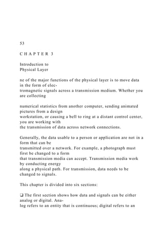
Figure 3.1 shows a scenario in which a scientist working in a research company, Sky
Research, needs to order a book related to her research from an online bookseller, Sci-
entific Books.
We can think of five different levels of communication between Alice, the com-
puter on which our scientist is working, and Bob, the computer that provides online ser-
vice. Communication at application, transport, network, or data-link is logical;
communication at the physical layer is physical. For simplicity, we have shown only
Figure 3.1 Communication at the physical layer
Alice
Sky Research
Scientific Books
Alice
R1 R2
R2
R3 R4
R4
To other
ISPs
To other
ISPs
R5
R5
R6 R7
R7
Bob
Bob
National ISP
Switched
WAN
ISP
Application
Transport
Network
D.
53C H A P T E R 3Introduction toPhysical Layern.docx
1. 53
C H A P T E R 3
Introduction to
Physical Layer
ne of the major functions of the physical layer is to move data
in the form of elec-
tromagnetic signals across a transmission medium. Whether you
are collecting
numerical statistics from another computer, sending animated
pictures from a design
workstation, or causing a bell to ring at a distant control center,
you are working with
the transmission of data across network connections.
Generally, the data usable to a person or application are not in a
form that can be
transmitted over a network. For example, a photograph must
first be changed to a form
that transmission media can accept. Transmission media work
by conducting energy
along a physical path. For transmission, data needs to be
changed to signals.
This chapter is divided into six sections:
❑ The first section shows how data and signals can be either
analog or digital. Ana-
log refers to an entity that is continuous; digital refers to an
2. entity that is discrete.
❑ The second section shows that only periodic analog signals
can be used in data
communication. The section discusses simple and composite
signals. The attri-
butes of analog signals such as period, frequency, and phase are
also explained.
❑ The third section shows that only nonperiodic digital signals
can be used in data
communication. The attributes of a digital signal such as bit
rate and bit length are
discussed. We also show how digital data can be sent using
analog signals. Base-
band and broadband transmission are also discussed in this
section.
❑ The fourth section is devoted to transmission impairment.
The section shows how
attenuation, distortion, and noise can impair a signal.
❑ The fifth section discusses the data rate limit: how many bits
per second we can
send with the available channel. The data rates of noiseless and
noisy channels are
examined and compared.
❑ The sixth section discusses the performance of data
transmission. Several channel
measurements are examined including bandwidth, throughput,
latency, and jitter.
Performance is an issue that is revisited in several future
chapters.
O
3. Data Communications and Networking, Fifth Edition 63
54 PART II PHYSICAL LAYER
3.1 DATA AND SIGNALS
Figure 3.1 shows a scenario in which a scientist working in a
research company, Sky
Research, needs to order a book related to her research from an
online bookseller, Sci-
entific Books.
We can think of five different levels of communication between
Alice, the com-
puter on which our scientist is working, and Bob, the computer
that provides online ser-
vice. Communication at application, transport, network, or data-
link is logical;
communication at the physical layer is physical. For simplicity,
we have shown only
Figure 3.1 Communication at the physical layer
Alice
Sky Research
Scientific Books
Alice
R1 R2
R2
4. R3 R4
R4
To other
ISPs
To other
ISPs
R5
R5
R6 R7
R7
Bob
Bob
National ISP
Switched
WAN
ISP
Application
Transport
Network
Data-link
Physical
6. CHAPTER 3 INTRODUCTION TO PHYSICAL LAYER 55
host-to-router, router-to-router, and router-to-host, but the
switches are also involved in
the physical communication.
Although Alice and Bob need to exchange data, communication
at the physical
layer means exchanging signals. Data need to be transmitted and
received, but the
media have to change data to signals. Both data and the signals
that represent them can
be either analog or digital in form.
3.1.1 Analog and Digital Data
Data can be analog or digital. The term analog data refers to
information that is
continuous; digital data refers to information that has discrete
states. For example, an
analog clock that has hour, minute, and second hands gives
information in a continuous
form; the movements of the hands are continuous. On the other
hand, a digital clock
that reports the hours and the minutes will change suddenly
from 8:05 to 8:06.
Analog data, such as the sounds made by a human voice, take on
continuous values.
When someone speaks, an analog wave is created in the air.
This can be captured by a
microphone and converted to an analog signal or sampled and
converted to a digital
signal.
7. Digital data take on discrete values. For example, data are
stored in computer
memory in the form of 0s and 1s. They can be converted to a
digital signal or modu-
lated into an analog signal for transmission across a medium.
3.1.2 Analog and Digital Signals
Like the data they represent, signals can be either analog or
digital. An analog signal
has infinitely many levels of intensity over a period of time. As
the wave moves from
value A to value B, it passes through and includes an infinite
number of values along its
path. A digital signal, on the other hand, can have only a
limited number of defined
values. Although each value can be any number, it is often as
simple as 1 and 0.
The simplest way to show signals is by plotting them on a pair
of perpendicular
axes. The vertical axis represents the value or strength of a
signal. The horizontal axis
represents time. Figure 3.2 illustrates an analog signal and a
digital signal. The curve
representing the analog signal passes through an infinite number
of points. The vertical
lines of the digital signal, however, demonstrate the sudden
jump that the signal makes
from value to value.
Figure 3.2 Comparison of analog and digital signals
Value
a. Analog signal
8. Time
Value
b. Digital signal
Time
Data Communications and Networking, Fifth Edition 65
56 PART II PHYSICAL LAYER
3.1.3 Periodic and Nonperiodic
Both analog and digital signals can take one of two forms:
periodic or nonperiodic
(sometimes referred to as aperiodic; the prefix a in Greek means
“non”).
A periodic signal completes a pattern within a measurable time
frame, called a
period, and repeats that pattern over subsequent identical
periods. The completion of
one full pattern is called a cycle. A nonperiodic signal changes
without exhibiting a pat-
tern or cycle that repeats over time.
Both analog and digital signals can be periodic or nonperiodic.
In data communi-
cations, we commonly use periodic analog signals and
nonperiodic digital signals, as
we will see in future chapters.
3.2 PERIODIC ANALOG SIGNALS
9. Periodic analog signals can be classified as simple or
composite. A simple periodic
analog signal, a sine wave, cannot be decomposed into simpler
signals. A composite
periodic analog signal is composed of multiple sine waves.
3.2.1 Sine Wave
The sine wave is the most fundamental form of a periodic
analog signal. When we
visualize it as a simple oscillating curve, its change over the
course of a cycle is smooth
and consistent, a continuous, rolling flow. Figure 3.3 shows a
sine wave. Each cycle
consists of a single arc above the time axis followed by a single
arc below it.
A sine wave can be represented by three parameters: the peak
amplitude, the fre-
quency, and the phase. These three parameters fully describe a
sine wave.
In data communications, we commonly use
periodic analog signals and nonperiodic digital signals.
Figure 3.3 A sine wave
We discuss a mathematical approach to sine waves in Appendix
E.
Time
Value
• • •
66 Computer Networking
10. CHAPTER 3 INTRODUCTION TO PHYSICAL LAYER 57
Peak Amplitude
The peak amplitude of a signal is the absolute value of its
highest intensity, propor-
tional to the energy it carries. For electric signals, peak
amplitude is normally measured
in volts. Figure 3.4 shows two signals and their peak
amplitudes.
Example 3.1
The power in your house can be represented by a sine wave with
a peak amplitude of 155 to 170 V.
However, it is common knowledge that the voltage of the power
in U.S. homes is 110 to 120 V.
This discrepancy is due to the fact that these are root mean
square (rms) values. The signal is
squared and then the average amplitude is calculated. The peak
value is equal to 21/2 × rms
value.
Example 3.2
The voltage of a battery is a constant; this constant value can be
considered a sine wave, as we
will see later. For example, the peak value of an AA battery is
normally 1.5 V.
Period and Frequency
Period refers to the amount of time, in seconds, a signal needs
11. to complete 1 cycle.
Frequency refers to the number of periods in 1 s. Note that
period and frequency are just
one characteristic defined in two ways. Period is the inverse of
frequency, and frequency
is the inverse of period, as the following formulas show.
Figure 3.5 shows two signals and their frequencies. Period is
formally expressed in
seconds. Frequency is formally expressed in Hertz (Hz), which
is cycle per second.
Units of period and frequency are shown in Table 3.1.
Figure 3.4 Two signals with the same phase and frequency, but
different amplitudes
f 5 and T 5
Frequency and period are the inverse of each other.
a. A signal with high peak amplitude
b. A signal with low peak amplitude
Peak
amplitude
Peak
amplitude
Time
Amplitude
• • •
12. Time
Amplitude
• • •
1
T
--- 1
f
---
Data Communications and Networking, Fifth Edition 67
58 PART II PHYSICAL LAYER
Example 3.3
The power we use at home has a frequency of 60 Hz (50 Hz in
Europe). The period of this sine
wave can be determined as follows:
This means that the period of the power for our lights at home is
0.0116 s, or 16.6 ms. Our
eyes are not sensitive enough to distinguish these rapid changes
in amplitude.
Example 3.4
Express a period of 100 ms in microseconds.
13. Solution
From Table 3.1 we find the equivalents of 1 ms (1 ms is 10–3 s)
and 1 s (1 s is 106 μs). We make
the following substitutions:
Figure 3.5 Two signals with the same amplitude and phase, but
different frequencies
Table 3.1 Units of period and frequency
Period Frequency
Unit Equivalent Unit Equivalent
Seconds (s) 1 s Hertz (Hz) 1 Hz
Milliseconds (ms) 10–3 s Kilohertz (kHz) 103 Hz
Microseconds (μs) 10–6 s Megahertz (MHz) 106 Hz
Nanoseconds (ns) 10–9 s Gigahertz (GHz) 109 Hz
Picoseconds (ps) 10–12 s Terahertz (THz) 1012 Hz
14. T 5 5 5 0.0166 s 5 0.0166 3 103 ms 5 16.6 ms
100 ms 5 100 3 10–3 s 5 100 3 10–3 3 106 ms 5 102 3 10–3 3
106 ms 5 105 ms
1 s
1 s
Time
Amplitude
a. A signal with a frequency of 12 Hz
b. A signal with a frequency of 6 Hz
Frequency is 12 Hz12 periods in 1 s
• • •
T
Time
15. Amplitude Frequency is 6 Hz6 periods in 1 s
• • •
Period: s112
Period: s16
1
f
--- 1
60
------
68 Computer Networking
CHAPTER 3 INTRODUCTION TO PHYSICAL LAYER 59
Example 3.5
The period of a signal is 100 ms. What is its frequency in