Downloaded 38 times


![3
new approach required a predictive mechanism (Kalman Filter) to allocate resources and
preemptively interact with network layers. Our results indicate that the improved
protocol raised the performance of Mobile IP in at least 30%.
We now define several concepts found in mobile networks and describe the rest
of the structure followed in this dissertation.
Concepts on Mobile Networks
Mobile networks challenge current paradigms of computing with varying
environments and scenarios characterized by sudden changes in bandwidth, error rates,
and latency for applications and system operations. Nomadic data in portable devices
make the current network protocols run short and supply insufficient solutions to solve
the mobility conditions of the new environment.
A few years ago, the network infrastructure was a fixed variable that seldom
changed. Although this assumption was totally accurate for Local and Wide-area
Networks (LAN and WAN), it is obsolete for wireless situations. In fact, wireless
networks incorporate the user experience with a set of services and benefits derived from
the pervasive environment. Additionally, a wide variety of settings and conditions exist
while roaming among different localities or moving across different areas covered by the
wireless infrastructure. These new attributes derived from the network conditions require
adaptive protocols to be able to adjust themselves and allows the seamless offering of
uninterrupted services to client applications, as currently provided in a fixed network.
Mobile users are nomadic since they connect from different access points during
the same network session and remain attached to the network while moving at any speed
within the globe, campus, or office. Furthermore, users move while network resources
(such as battery life and wireless bandwidth) are limited [Jin99]. Protocols should adapt](https://image.slidesharecdn.com/hernandezefinal-100909142132-phpapp01/85/Adaptive-Networking-Protocol-for-Rapid-Mobility-16-320.jpg)
![4
and provide nondisruptive connectivity to the mobile users. This adaptation process
requires predictable mechanisms and awareness of the physical conditions. In general, the
physical layer is aware of the changing media conditions. Some characteristics are
already detected in the lower layers of the stack. In fact when important changes happen
at a lower layer, they are usually hidden from higher layers [Sone01, Wu01]. Therefore,
information exchange between upper and lower layers of the stack is a key factor for
mobile networks. Additionally, knowledge of mobile user movement and connection
patterns can improve the session quality by predicting trajectories and allocating network
resources before they are required. Proper predictive strategies can indeed reduce the
requirements of network updates and handoff delays [Liu98, Lia99, and Su00]. Physical
parameters can also be used to locate users, track their position within different network
cells and develop new location management strategies [Bahl00b].
Network-layer mobility is not supported by default in the Internet Protocol (IP)
and the traditional implementations of the Transport Control Protocol (TCP) are unable to
distinguish between handoff and congestion avoidance [Bala96, Jaco88]. In fact, the
Internet protocol suite was designed under the assumption that end systems are
stationary. Thus, as one network end moves, the network session is broken [Bha96]. For
the operating system, the session simply times out, and new kernel bindings are required
to support mobility.
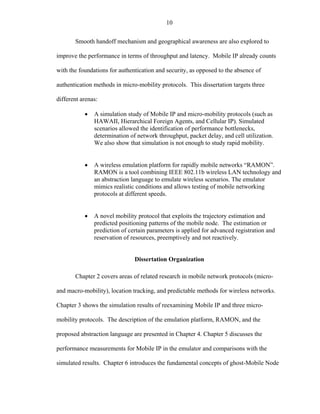
Network-layer mobility has been improved by the use of registered stations taking
care of the routing and forwarding of packets which destination is currently moving
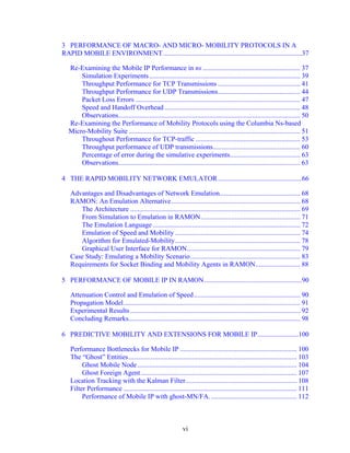
[Bha96]. Mobile IP [Perk96a, Perk96b, and Perk02] is one of the proposed solutions
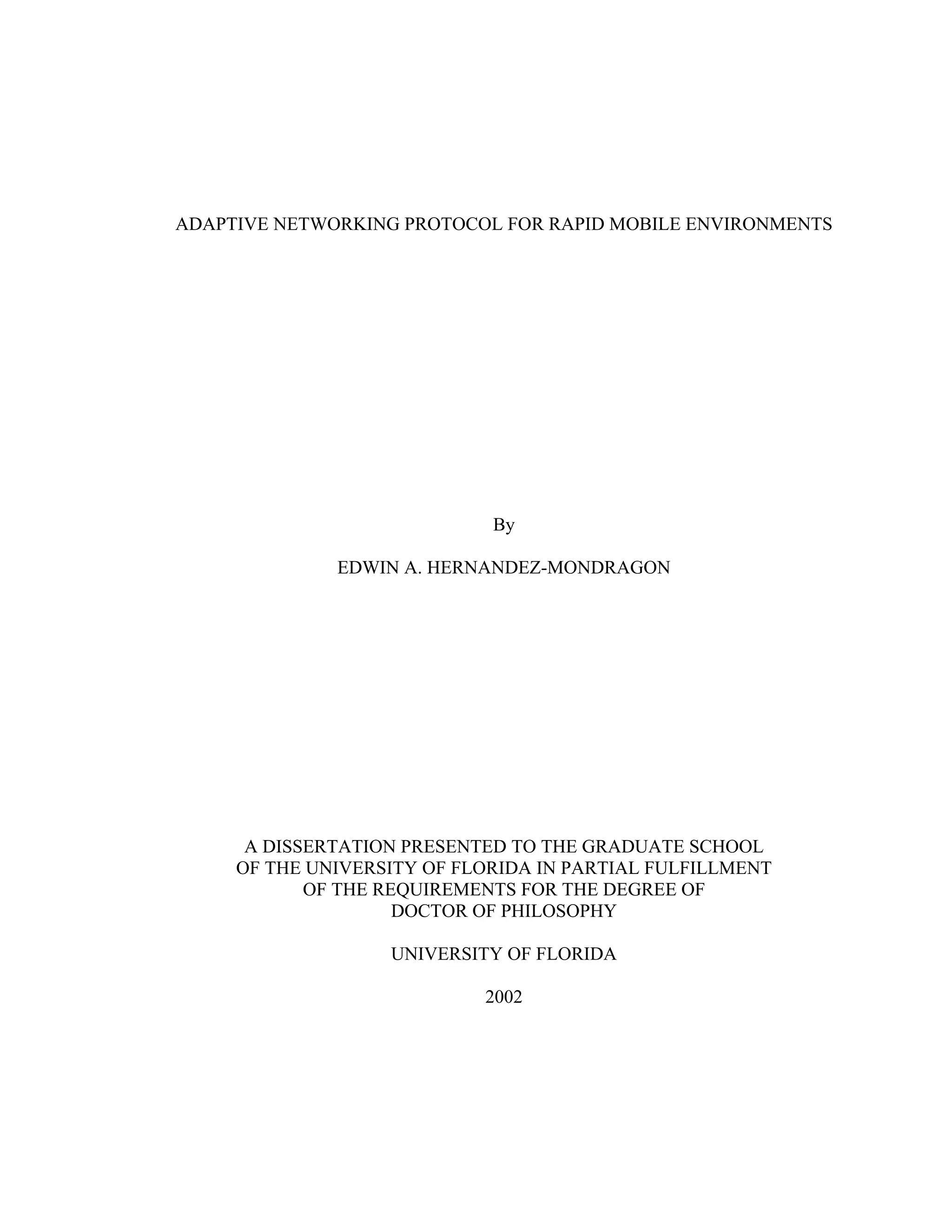
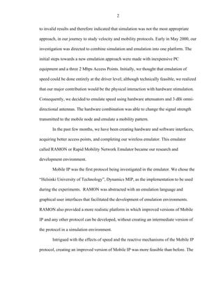
based on registration and packet forwarding. As shown in Figure 1, Mobile IP for IPv4](https://image.slidesharecdn.com/hernandezefinal-100909142132-phpapp01/85/Adaptive-Networking-Protocol-for-Rapid-Mobility-17-320.jpg)
![5
and IPv6 required of an entity called Home Agent (HA), who registers the position of the
Mobile Host (MH). Similar registration mechanisms can be found in the standard for
Global Systems for Mobile Communications (GSM), where the Home Location Register
(HLR) [Hill02] acts as the registration entity to maintain updated position and routing
information for the mobile nodes.
Home
network
Stationary
host
Internet routing
Foreign Network
Figure 1. Mobility scenario from a home to a foreign network
The mobile node communicates with a destination node which can be a web- or
multimedia-based server also denominated as the Correspondent Host (CH). Once the
Correspondent Host (CH) sets a communication link with the MH, the registration
service at the HA intermediates the requests and encapsulates the packets coming from
the CH to the proper registration destiny found in its directory. Therefore, the MH must
update the HA continuously with the current information of the foreign network being
visited. The foreign network designates another entity, the Foreign Agent (FA), to
exchange information between the MH and the foreign network.
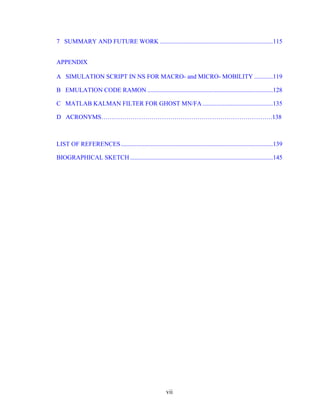
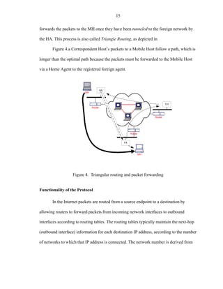
As in Mobile IP, GSM networks counts with a Visitor Location Register (VLR) to
take care of the role of the FA. Indeed, a generalization of the different network
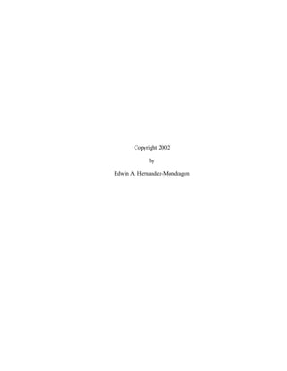
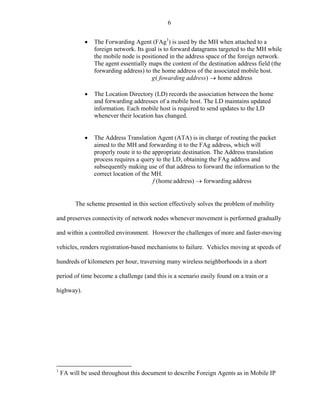
components used for the mobility environment is shown in Figure 2. [Bha96]. Those
components are:](https://image.slidesharecdn.com/hernandezefinal-100909142132-phpapp01/85/Adaptive-Networking-Protocol-for-Rapid-Mobility-18-320.jpg)
![7
Location Directory
Home LD
network
Address Translation Agent
Foreign Network
Source f Forwarding Agent
g
Cache
Internet routing
MH
f: Home Address Forwarding Address
g: Forwarding Address Home Address
Figure 2. Packet forwarding model
Rapidly Moving Environments
The proliferation of wireless networks and high-speed internet access for the
transportation industry can be implemented with today’s technology and the use of
current Wi-Fi access points and network cards. Wi-Fi provides connection speeds of 1-
11Mbps [Bing00] and represents a potential option for the deployment of internet
connectivity on highways and train tracks. While 3G presents a promising solution for
future wireless subscribers, the bandwidth offered in 3G networks (CDMA200) for
vehicular speeds is in the range of 140 Kbps [Garg00]; consequently higher deployment
and licensing costs are expected. Vehicular routes of trains and highways can benefit
from Wireless LANs and supply end users with a communication scenario similar to
existing office and home environments (without expenditures on extra equipment or
technologies).
As mentioned in the previous section, the mainstream solution for network-layer
mobility is solved by registering the movement of the mobile node to a centralized
database of location information or the Location Directory (LD). Although centralized
databases ease the solution for problems of authentication, accounting, and authorization](https://image.slidesharecdn.com/hernandezefinal-100909142132-phpapp01/85/Adaptive-Networking-Protocol-for-Rapid-Mobility-20-320.jpg)
![8
of mobile users in the network [Glass00], the LD might not be suitable for vehicular
applications. In fact, an LD might contain expired information of an MH already moved
to a different location, or cell, or the network delay might be intrinsically close or higher
than the dwell time of the MH. A solely registration-based solution is not a suitable for
rapidly moving environments [Hern01].
Indeed, registration mechanisms represent a major obstacle for a wide deployment
of wireless networks in vehicular applications. The wireless technologies: IEEE 802.11a
and IEEE 802.11b [Ieee99a, Ieee99b] offer micro-cell coverage, high throughput, and
cheap deployment. The combination of these factors and the native characteristics of
Mobile IP metrics: network delay, handoff speeds, and the packet-forwarding entail of an
alternative approach bound for a less dependent registration protocol.
In 802.11x, cells sizes from 50 to 1000 m, depending upon the throughput and
latency of the wireless technology in use. For example, 802.11b a network cell ranges
[Cis01] from 200 to 1000 m for indoor and outdoor environments, providing throughputs
of 1 to 11 Mbps. In fact, a cell diameter of 400 m and a mobile unit at 80 m/s generate a
dwell time of 5 s. Any authentication mechanism, network delay, or handoff initiated at
the mobile host will diminish the performance and use of the cell significantly by
assuming processing times on the order of one second (20% of the dwell time on the cell
at this speed). There is a trend for cell sizes to decrease in diameter (down to 50 m) while
network throughput increases to a range of 50-100 Mbps as described in the IEEE
802.11a standard. As a result, the mobility protocol in use (e.g. Mobile IP) requires
architecture and mobility awareness to adapt to the changing conditions of mobility.](https://image.slidesharecdn.com/hernandezefinal-100909142132-phpapp01/85/Adaptive-Networking-Protocol-for-Rapid-Mobility-21-320.jpg)

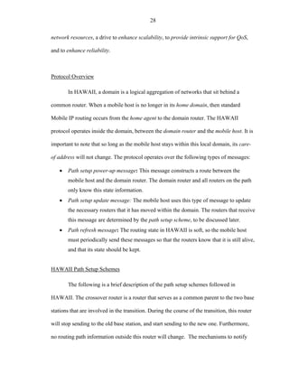
![CHAPTER 2
RELATED RESEARCH
This chapter introduces the concepts and protocols used for mobility at a Macro-
and Micro-levels. Mobile IP and hierarchical Foreign Agents are presented as part of
Macro-mobility models followed by Cellular IP and HAWAII as micro-mobility
protocols. In addition, we introduce several research remarks in terms of geographic
routing use and the effects of speed on macro-mobility protocols.
Mobile IP
Mobile IP (RFC 2002) [Perk96a, Perk02] a standard proposed by one of the
working groups within the Internet Engineering Task Force (IETF), was designed to
solve the problem of mobility by allowing the mobile node to use two IP addresses: a
fixed home address and a care-of address that changes at each new point of attachment.
As shown in Figure 3 the home network provides the mobile node with an IP address and
once the node moves to a different network it receives a care-of-address assigned by the
foreign network.
The version of Mobile IP described in this section corresponds to IP version 4,
however Mobile IP will change with IP version 6 [Perk96a], which is the product of a
major effort within the IETF to engineer an eventual replacement for the current version
of IP. Although IPv6 will support mobility to a greater degree than IPv4, it will still need
Mobile IP to make mobility transparent to applications and higher-level protocols such as
12](https://image.slidesharecdn.com/hernandezefinal-100909142132-phpapp01/85/Adaptive-Networking-Protocol-for-Rapid-Mobility-25-320.jpg)
![13
TCP. The following subsections will present the features of Mobile IP, and
supplementary definitions that are used throughout this proposal, as well as a description
of the protocol functionality.
Foreign
Agent
S MH MH
R4
d Home d
Agent
R1 R2 R3
Figure 3. IETF proposal for mobility
Features of Mobile IP
The IETF proposal has become the most popular protocol for handling mobility in
the Internet. Mobile IP was designed with the following characteristics:
• No geographical limitations, in other words a user can take a PDA or laptop
computer anywhere without losing the connection to the home network.
• No physical connection is required for mobile IP while the mobile node
determines local IP routers and connects automatically.
• Modifications to other routers and hosts are not required as in many micro-
mobility protocols. Indeed, other than mobile nodes and agents, the remaining
routers and hosts will still use current IP implementation. Mobile IP leaves
transport and higher protocols unaffected.
• No modifications to the current IP address and IP address format are required;
the current IP address format remains the same.
• Secure mobility, since Authentication, Accounting, and Authorization (AAA)
[Glas00] are performed at a centralized location, mobile IP can ensure that
rights are being protected.](https://image.slidesharecdn.com/hernandezefinal-100909142132-phpapp01/85/Adaptive-Networking-Protocol-for-Rapid-Mobility-26-320.jpg)
![14
Definitions and Terminology
There are several definitions and terms defining the mobile IP standard. First of
all a Host is any computer, not considered to be performing routing or bridging functions
while a Mobile Host (MH) represents a host that moves from place to place, indeed static
placement of computers becomes a non-valid assumption. Moreover a Correspondent
Host (CH) is a server or a station from the fixed or wired network that communicates
with another MH.
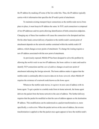
The protocol also defines two types of addresses, the first one Home Address is
used to identify a Mobile Host in general the IP address originally assigned to the MH
either using Dynamic Host Configuration Protocol (DHCP) [Perk95] or manually
configured, while the second address corresponds to a Foreign Address which is used to
locate a Mobile Host at some particular instant of time at a different location or while
visiting a different network. Both addresses can be obtained using a DHCP server or any
other type of assignment done at the home or foreign networks.
Since we count with a home and a foreign address, there are two entities in charge
of the home and the foreign networks. The Home Agent (HA), located at the home
network, redirects or tunnels packets from a Home Network to a Foreign Address of a
Mobile Host. Hence, the Home Network is the logical network on which a Mobile Host’s
Home Address resides. The second entity in this architecture corresponds to a Foreign
Agent (FA), located in the foreign network, offers a Foreign Address and performs a
mapping between that address and the Home Address of a Mobile Host. The FA also](https://image.slidesharecdn.com/hernandezefinal-100909142132-phpapp01/85/Adaptive-Networking-Protocol-for-Rapid-Mobility-27-320.jpg)
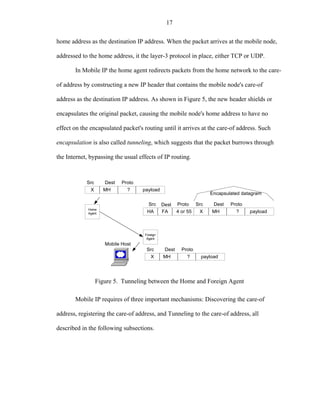
![19
security, the mobile node and home agent share a security association and so are able to
use MD5. The registration request must contain unique data so that two different
registrations will in practical terms never have the same MD5 hash.
The triplet that contains the home address, care-of address, and registration
lifetime is called a binding for the mobile node. A registration request can be considered
a binding update sent by the mobile node. See Figure 6.
MH FA HA
Send Solicitacions
Send Advertisements
Update Agent List
Handoff necessary
Registration Request
Forwarding Request
Registration Reply
Forwarding Reply
New COA
Figure 6. Handoff and re-registration in Mobile IP [Widm00]
Tunneling to the Care-Of-Address
The default encapsulation mechanism that must be supported by all mobility
agents using Mobile IP is IP-within-IP. Using IP-within-IP, the home agent inserts a new
IP header, called the tunnel header, in front of the IP header of any datagram addressed to
the mobile node's home address. The new tunnel header uses the mobile node's care-of
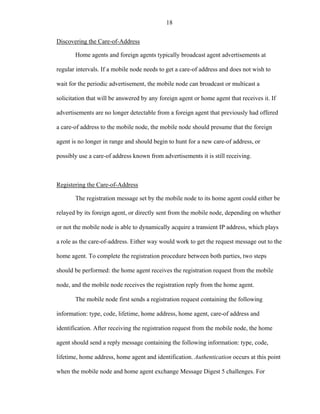
address as the destination IP address, or tunnel destination. The tunnel source IP address](https://image.slidesharecdn.com/hernandezefinal-100909142132-phpapp01/85/Adaptive-Networking-Protocol-for-Rapid-Mobility-32-320.jpg)
![20
is the home agent, and the tunnel header uses the number 4 as the higher-level protocol
number, indicating that the next protocol header is again an IP header. In IP-within-IP,
the entire original IP header is preserved as the first part of the payload of the tunnel
header. Therefore, to recover the original packet, the foreign agent merely has to
eliminate the tunnel header and deliver the rest to the mobile node.
In a special case sometimes the tunnel header uses protocol number 55 as the
inner header. This happens when the home agent uses minimal encapsulation instead of
IP-within-IP. Processing for the minimal encapsulation header is slightly more
complicated than that for IP-within-IP, because some of the information from the tunnel
header is combined with the information in the inner minimal encapsulation header to
reconstitute the original IP header. On the other hand, header overhead is reduced.
Figure 7. Tunneling using IP-in-IP encapsulation and minimal encapsulation [Solo98]](https://image.slidesharecdn.com/hernandezefinal-100909142132-phpapp01/85/Adaptive-Networking-Protocol-for-Rapid-Mobility-33-320.jpg)
![21
Route Optimization in Mobile IP
IPv6 mobility borrows heavily from the route optimization ideas specified for
IPv4, [Perk01] particularly the idea of delivering binding updates directly to
correspondent nodes. When it knows the mobile node's current care-of address, a
correspondent node can deliver packets directly to the mobile node's home address
without any assistance from the home agent. Route optimization is likely to dramatically
improve performance for IPv6 mobile nodes. It is realistic to require this extra
functionality of all IPv6 nodes for two reasons. First, on a practical level, IPv6 standards
documents are still at an early stage of standardization, so it is possible to place additional
requirements on IPv6 nodes. Second, processing binding updates can be implemented as
a fairly simple modification to IPv6's use of the destination cache.
Hierarchical Foreign Agents
Frequent handoff may produce constant packet loss due to the registration process
and before the next care-of-address is obtained by the mobile host. Speed aggravates this
performance problem. Hierarchical Foreign Agents [Perk96b, Cast98] (HFA) focuses on
the alleviation of this problem by organizing the FAs in a domain area with certain
hierarchy, more precisely a tree of FAs in order to handle local movement within a
domain. As shown in Figure 8 to handle local movements within a domain the MH
chooses a closer registration point. The architecture requires traversing only a factor of
log(N) of FAs in order to register the binding update, where N corresponds to the number
of FAs in the network. However, the number of elements per domain increases
exponentially such that 2M-1 additional routers are required per domain with M cells.](https://image.slidesharecdn.com/hernandezefinal-100909142132-phpapp01/85/Adaptive-Networking-Protocol-for-Rapid-Mobility-34-320.jpg)
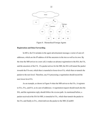
![23
Handoff Management
During Handoff, the MH compares the new vector of care-of-addresses with the
old one. Again, it chooses the lowest level address of the FA that appears in both-vectors
and sends a Regional Registration Request, which is processed by the FA. There is no
need to notify any higher-level FA about this handoff since those FA already points to the
proper location where to tunnel the packets for the MH. In Figure 8, the MH sends a
regional registration message to FA3, FA1 and the HA still maintains the proper
destination. When the MH moves to FA5 then it requires to the FA1, although several
handoffs have occurred the HA has not required to be updated and therefore the
registration overhead is greatly reduced.
Micro-Mobility Protocols
Macro-mobility protocols introduce high overhead in terms of registration
messages, tunneling, triangular routing, and hard-handoff mechanisms. Several research
efforts [Camb01, Camb02, Ramj01] have improved the performance of Mobile IP by
creating domains of mobility where macro-mobility is executed at the level of inter-
domain handoff, while intra-domain is handled locally without intervention of the HA
and FAs.
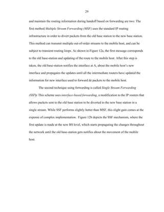
Figure 9 depicts the micro-mobility model used by Cellular IP and HAWAII and
how the network infrastructure manages handoff within the local domain while the inter-
domain handoff is taken care by the Mobile IP protocol. Additionally, micro-mobility
protocols provide paging information, as well as QoS mechanisms at the domain level.](https://image.slidesharecdn.com/hernandezefinal-100909142132-phpapp01/85/Adaptive-Networking-Protocol-for-Rapid-Mobility-36-320.jpg)
![24
In general micro-mobility protocols provide a highly optimized routing mechanism, with
memory less support for mobility and smoother handoffs.
The following two sub-sections describe two micro-mobility protocols found in
the literature.
CH
Network
Home Domain
Router HA FA Foreign Domain
Router
root root
home domain foreign domain
Movement between domains, HA is notified
MH
Movement within domain, Movement within domain,
HA not involved HA not involved
Figure 9. Micro-mobility architecture [Camp01]
Cellular IP
Although Mobile IP meets the goals of operational transparency and handoff
support, it is only optimized for slowly moving hosts and becomes inefficient in the case
of frequent migration. Mobile IP requires that the mobile hosts’ home agent be informed
whenever the host moves to a new Foreign Agent. During the update message phase,
packets will be forwarded to the old location and will not be delivered hence disturbing
active data transmission. In general Mobile IP is optimized for macro-level mobility and](https://image.slidesharecdn.com/hernandezefinal-100909142132-phpapp01/85/Adaptive-Networking-Protocol-for-Rapid-Mobility-37-320.jpg)
![25
relatively slow-moving hosts and hence results in huge delays with increasing handoff
frequency.
Cellular IP [Camp01] is a host mobility protocol that is optimized for wireless
access networks and highly mobile hosts. Cellular IP incorporates a number of important
cellular principles but remains firmly based on IP design principles allowing Cellular IP
to scale from pico- to metropolitan area installations.
The main design motivations for Cellular IP protocol are:
• Easy global migration;
• Cheap passive connectivity;
• Flexible handoff support;
• Efficient location management;
• Simple memory less mobile host behavior
Routing
Uplink packets are routed from mobile to the gateway on a hop-by-hop basis. The
path taken by these packets is cached in base stations. To route downlink packets
addressed to a mobile host the path used by recent packets transmitted by the host is
reversed. Base stations record the interface that was used earlier and use it to route
packets toward the gateway. As these packets are routed toward the gateway their route
information is recorded in the route cache. In the scenario illustrated in Figure 5 data
packets are transmitted by a mobile host with IP address X and enter BS2 through its
interface a. In the routing cache of BS2 this is indicated by a mapping (X,a).
Handoff
There are two kinds of handoff in cellular IP: Hard and semi-soft handoff. The
first mechanism, hard handoff, requires the mobile host to tunes its radio to the new base
station and sends a route-update packet. There is latency equal to the time that elapses](https://image.slidesharecdn.com/hernandezefinal-100909142132-phpapp01/85/Adaptive-Networking-Protocol-for-Rapid-Mobility-38-320.jpg)
![26
between the handoff and the arrival of the first packet through the new route, which
causes some packet loss.
Correspondant
host
Home
Mobile IP Agent
Internetworking
R
IP routing
IP tunneling
Cellular IP routing BS4
BS2
b
BS1
a
Mobile X
BS3
Mobile X
Figure 10. Routing mechanism on Cellular IP [Valk99]
The second type of handoff, semi-soft handoff, in order to reduce the latency
involved, the mobile host sends a “semi-soft packet” and reverts back to the old base
station while route cache mappings are configured. Once the configuration is completed a
regular handoff takes place ensuring that there is no packet loss.
Figure 11. Handoff in Cellular IP [Camp02]](https://image.slidesharecdn.com/hernandezefinal-100909142132-phpapp01/85/Adaptive-Networking-Protocol-for-Rapid-Mobility-39-320.jpg)
![27
Paging
Paging occurs when a packet is addressed to an idle mobile host and the gateway
or base stations find no valid routing cache mapping for the destination. It is used to
avoid broadcast search procedures found in cellular systems. Base stations optionally
maintain paging cache to support paging. The paging cache has the same format as
routing cache except that the cache mappings have a longer timeout and they are updated
by any packet sent by mobile hosts including paging-update packets.
HAWAII
In addition to Cellular IP and the deficiencies found in Mobile IP, Ramjee, et al.
proposed HAWAII (Handoff-Aware Wireless Access Internet Infrastructure) [Ramj99,
Ramj00] as an extension to Mobile IP that corrects the following deficiencies:
• In Mobile IP, user traffic is disrupted when the mobile host changes domains.
• In Mobile IP, costly updates to the home agent must be made for every
domain change.
• When mobile hosts change domains, they acquire new network paths to the
home agent. In turn, this requires the old QoS guarantee to be torn down, and a
new one (along the new route) to be established. Because these QoS setups are
costly, they should be minimized.
• The requirements for home and foreign agents incur a robustness penalty. This
penalty should be reduced.
Essentially, HAWAII attempts to improve Mobile IP performance by making the
assumption that most of the mobility is within a single logical administrative domain
which may be composed of many physical sub-domains. The HAWAII protocol is driven
by five design goals: limit the disruption to user traffic, enable the efficient use of access](https://image.slidesharecdn.com/hernandezefinal-100909142132-phpapp01/85/Adaptive-Networking-Protocol-for-Rapid-Mobility-40-320.jpg)
![32
forwarding mode corresponds to the same value as in Cellular IP or the time to reach the
cross-over router.
In terms of latency, semi- and hard-handoff provide an average delay of 2Tg, or
the time to reach the gateway, while in HAWAII in average 2Thoffb
Geographical-Based routing
Applications based on Geographical Position Systems (GPS) and Geographical
Information Systems (GIS) are heavily used by civil engineers. The same tools and
concepts can be also reused for location tracking of mobile nodes.
Location Aided routing (LAR) [Ko98] assumes that GPS information is available
during routing in ad-hoc networks, additionally the use of GPS and Mobile IP [Erge02]
have shown improvements during handoff and registration. Other existing protocols such
as GeoCast [Nav97] use similar mechanisms for positioning and geographical addressing
during data delivery.
GPS systems are expensive and consume battery power which might also be
required for the network card in a mobile unit. Indirect location determination has also de
determined through the measurement of signal strength and signal-to-noise ratio. The
RADAR project, research conducted at Microsoft Research by Bahl, et al. [Bahl00a,
Bahl00b], is an effort to provide location tracking and management for Wireless
Networks based on IEEE 802.11x using the signal strength level. This research initiative
is an example of how physical media information can be used to determine positioning
information of a mobile unit within an office environment. The location information is
calculated based on triangulation of the signal strength and IEEE 802.11 context
information.](https://image.slidesharecdn.com/hernandezefinal-100909142132-phpapp01/85/Adaptive-Networking-Protocol-for-Rapid-Mobility-45-320.jpg)
![33
Many tracking systems use geographical information to page mobile users and
allocate resources in advance which in general improves the quality of service offered in
the wireless environment. RADAR uses signal strength information gathered at multiple
receiver locations to triangulate the user’s coordinates. In the RADAR system,
information regarding signal strength is gathered as a function of the user’s location.
The input parameters used in the RADAR project correspond to the Signal
Strength (SS) in dBm which is given by the relationship 10 log10 ( s / 0.001) where s is
given in Watts. In addition, the Signal-to-Noise Ratio (SNR) is calculated thru the
formula 10 log10 ( s / n) in dBm that is merged with the signal strength value to create a
database of SNR and SS values as a function of the user’s location.
Theoretical estimation of the distance between the transmitter and receiver can be
made by the path-loss equations proposed by Rappaport [Rapp02] using different
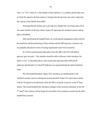
propagation models. As shown in Figure 13, the signal is transmitted by the base-station
node, the media or the geographical conditions produces certain attenuation and the noise
levels at the mobile node’s location is added to generate the current r(t) or received
measured signal strength.
Mobile protocols targeted for rapidly moving vehicles can receive a great benefit
from geographical information direct or indirect measures. Henceforth, Chapter 5 and 6
will describe the determination of position and the implementation of the adaptive
protocol.](https://image.slidesharecdn.com/hernandezefinal-100909142132-phpapp01/85/Adaptive-Networking-Protocol-for-Rapid-Mobility-46-320.jpg)
![34
r(t)
x(t)
Attenuation Model
RF transmitter n(t)
Figure 13. Signal propagation mode
Speed and Rapid Mobility
Speed has been researched mostly as part of ad-hoc networks and handoff rate is
usually related to infrastructure-based protocols. Speed could have a negative effect on
mobility, especially the performance of ad-hoc routing protocols. Holland, et al. [Holl99]
simulated several ad-hoc scenarios and showed that the average throughput decreases at
higher speeds. The results corresponded to a simulation performed in ns network
simulator [Fall00] focusing only on the performance of ad-hoc networks. The same
effects on throughput due to speed were measured by Gerla [Gerl99], while
experimenting with tree multicast strategies in ad-hoc networks at speeds up to 100
km/hr.
Fladenmuller [Flad99] analyzed the effect of Mobile IP handoffs on the TCP
protocol. The issues addressed in [Cace96a] involve handoff as a dual process taking
effect in the wired and wireless networks. Although, no quantitative considerations on the
speed of mobile nodes were presented, a conclusion was drawn in terms of the effect of
pico-cells and highly frequent handoff as the main factor to modify the TCP and Mobile
IP protocols. Similarly, Caceres [Cace96a, Cace96b] proposed fast-retransmissions as a
solution to solve the problems related to hand-off. Although his protocol improves the](https://image.slidesharecdn.com/hernandezefinal-100909142132-phpapp01/85/Adaptive-Networking-Protocol-for-Rapid-Mobility-47-320.jpg)
![35
performance of TCP, it does not assert the issue of speed and how the retransmission
timers could be modified or calculated.
Additionally, Balakrishnan [Bala95, Bala96] studied the protocols: Snoop, I-TCP
(Indirect TCP), and SACK (Selective acknowledgments). These protocols alleviate the
problems of TCP in wireless links and improve the performance during handoff. The first
protocol, called Snoop, is a software agent located at each base station, which attempts to
use multicast addresses to hide the location of mobile nodes. The second protocol, I-TCP
separates the wired and wireless links into two for the wireless and wired environments.
SACK has shown improvements in recovering from multiple packet losses within a
single transmission window. The results showed that these protocols improve the
performance of TCP under high BER (Bit Error Rate) links, and consequently can avoid
unnecessary activation of the congestion control protocol [Jaco88] during handoff. Again
I-TCP and SACK did not address the speed factor directly.
Predictable Mobility
Several approaches are found in the literature regarding predictable trajectory.
Liang and Hass [Lia99] provide a predictive-distance based location management
algorithm for a vehicle moving across two cells. Instead of a random walk model or
group mobility, their model provides a more realistic Gaussian-Markov state machine
where current user location is predicted given previous values of location and velocity.
Liu, et al. [Liu98] proposed a more complex predictive mechanism for mobility
management in W-ATM (Wireless Asynchronous Transfer Mode) networks. The
algorithm is based on a Kalman Filter and the commonly known Hierarchical Location
Prediction algorithm (HLP). The algorithm combines location updating with location
prediction for resource reservation and allocation in W-ATM networks. Similarly, Liu](https://image.slidesharecdn.com/hernandezefinal-100909142132-phpapp01/85/Adaptive-Networking-Protocol-for-Rapid-Mobility-48-320.jpg)
![36
used a Mobility Motion Prediction (MMP) algorithm with a pattern-matching using the
mobility patterns of the vehicles to estimate speed and improve handoff.
Acampora and Naghshineh [Aca94] suggest the Virtual Connection Tree (VCT)
architecture to provide and allocate enough resources for mobile hosts in the network.
This approach is very similar to HAWAII and Cellular IP in the sense that mobility
trajectory is not known by the base-stations and many resources are allocated whether
used or not.
Some other approaches to rapid mobility and predictable mobility include
dynamic programming and stochastic control [Reza95]. These approaches find the
optimal point while reducing the problem of handoff to a mobile node and two adjacent
cells. Their goal is to optimize the threshold of receive signal strength used for handoff
(based upon the mobility patterns and attenuation model)
Levine [Levi95] proposes the concept of shadow cluster where the surrounding
cells to a mobile node become a shadowing cluster and packets are forward to the cluster
depending upon network and mobility conditions. However it is not clear how the
probability matrices and mobility patterns is fed up to the system of base-stations.
Levine’s proposal follows our proposal of ghost Mobile IP described in Chapter 6.
Mobility prediction has also been a factor in Ad-hoc networks [Su00] where
predicting mobility based-upon GPS information shown improvement performance in
Distance Vector protocols.](https://image.slidesharecdn.com/hernandezefinal-100909142132-phpapp01/85/Adaptive-Networking-Protocol-for-Rapid-Mobility-49-320.jpg)
![37
CHAPTER 3
PERFORMANCE OF MACRO- AND MICRO- MOBILITY PROTOCOLS IN A
RAPID MOBILE ENVIRONMENT
The dissemination of mobile networks and the increasing demand for Internet
access in terrestrial vehicles makes commuter trains a suitable platform to provide
wireless access to the information superhighway. Internet applications such as browsing,
emailing, and audio/video streaming, currently common in wired networks, will be
demanded in this rapidly mobile environment. This translates to QoS requirements for
multimedia data from UDP- and TCP-based application sessions. Continuous
connectivity, responsiveness and steady throughput are among the important QoS
variables that have to be optimized throughout the train paths and trajectories. The first
sub-section presents the performance numbers of Mobile IP measured using the ns
network simulator [Hern01] and the CMU extensions for wireless networks [Mon98].
The second part of this chapter presents the experimental results for micro-mobility
protocols but using the IP-micro-mobility suite developed by Columbia University
[Valk99, Camb00] including performance values for Mobile IP, as well as Hierarchical
Foreign Agents and Celullar-IP. This chapter presents the simulative results made using
the ns using Mobile IP and the micro-mobility protocols.
Re-Examining the Mobile IP Performance in ns
Mobile IP [Perk96, Solo98] is the proposed standard for IP mobility support by
the Internet Engineering Task Force (IETF). The standard defines three entities: mobile
node, home agent, and foreign agent. Each mobile node has a permanent IP address](https://image.slidesharecdn.com/hernandezefinal-100909142132-phpapp01/85/Adaptive-Networking-Protocol-for-Rapid-Mobility-50-320.jpg)
![38
assigned to a home network, also called home address. Once the mobile node decides to
move away from its home network, the new location of the mobile host is determined by
the care-of-address, which is a temporary IP address from the foreign network. In
addition to the addressing procedures, the standard proposes a mobility binding method
between the mobile node, the home and foreign agents. The way IP packets are routed
from the correspondent host towards the mobile unit is through tunneling of the packets
by the home agent to the care-of-address, bound by the mobile host. Once the packet
arrives to the destination, the foreign agent proceeds to remove the encapsulated
information and forwards it to the mobile node. This process is also called triangular
routing.
This standard for mobility assumes relatively low speeds, which makes it very
suitable for macro-mobility and nomadic environments. However, high-speed commuter
trains move at speeds up to 288 Km/hr (0 to 80 m/s) which drastically reduces the
effectiveness of the Mobile IP protocol and diminishes the quality of its services.
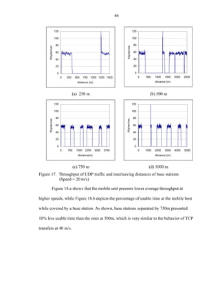
This section presents a performance analysis of Mobile IP under rapid mobility
conditions. We examine the effect of speed on throughput, delays, and packets drop rate
of UDP and TCP transfers. In our experiments, we manufacture speed as a product of two
factors: 1) the velocity of the mobile unit, and 2) the average (or fixed) interleaving
distance between base stations. We base our experiments on the IEEE 802.11 wireless
LAN technology [Ieee99a, Bing00], which represent the most appropriate MAC and
physical layers available today that can deliver high-speed services to commuter train
users (3G-NOW).](https://image.slidesharecdn.com/hernandezefinal-100909142132-phpapp01/85/Adaptive-Networking-Protocol-for-Rapid-Mobility-51-320.jpg)
![39
Simulation Experiments
The results in this paper are based on simulation experiments performed within
the ns network simulator from Lawrence Berkeley National Laboratory (LBNL) [Fall00],
with extensions from the MONARCH project at Carnegie Mellon/Rice University
[Mona98]. We made use of the IEEE 802.11 MAC layer implementation as our physical
transport layer. The mobile host and base stations were configured with the standard
mobile node features defined by ns. The experiments were classified by traffic type: a)
UDP and b) TCP. For UDP, a back-to-back randomly generated 532 bytes packet was
sent at a constant rate of 0.8 Mb/sec to a destination in a wired network. While TCP
transfers consisted of an FTP session executed from the mobile node to the wired
network. The standard TCP implementation was used throughout the experiments. We
measured the performance in the opposite direction and the differences between both
experiments were minimal and only results of the former are presented in this paper.
The network topology consisted of a set of base stations located at 250, 500, 750,
and 1000 meters away from each other, as depicted in Figure 14. The separation distance
between the base stations was considered an important experimental variable, provided
that at different speeds the mobile host will have different rendezvous periods with the
cell covered by a specific base station and that coverage area gaps might be present
throughout the train trajectory. In addition, infrastructure cost might be a factor that
requires certain spacing between base stations, and hence the importance of this variable.](https://image.slidesharecdn.com/hernandezefinal-100909142132-phpapp01/85/Adaptive-Networking-Protocol-for-Rapid-Mobility-52-320.jpg)
![40
INTERNET
1 1
1
1
1 1 gateway
Wired - nodes 5 Mb/2 ms
5 Mb/2 ms
v 2 Mb / 10 ms 2 Mb / 10 ms
Base Station N]
[
Home Agent Base Station [1]
Figure 14. Network topology for a train environment simulated with ns
The architecture depicted in Figure 14 represents a realistic design that may be
used to cover a railroad track of a train. All foreign agents share a bus instead of a star
topology, which is unrealistic. The links between base stations are of 2 Mb/s and 10 ms
delay, the wired links are 5 Mb/s and 2 ms delay connections. All traffic is generated
from the mobile node to the farthest wired node show in the figure. We simulated one
mobile host moving from the origin (the home network) towards a destination following
a straight line, traversing a set of foreign nodes at a constant speed ranging from 0 to 80
m/s. It is not practical to simulate more than one mobile node, since internally in each
compartment a different LAN might coexist and the simulation only represents a mobile-
bridge or a router conducting the traffic from all the mobile stations inside the train cars.
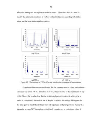
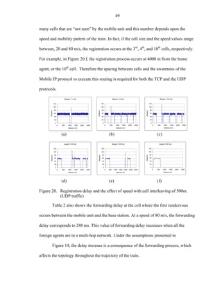
The main goal of this experimental study is to measure the effect of speed and the
interleaving of the base stations on the overall performance of the Mobile IP protocol.
The experiments, which were performed according to the topology presented in
Figure 14, measured the network throughput at the destination node, overall
packet loss, and the overhead generated during handoff. The overhead of the registration](https://image.slidesharecdn.com/hernandezefinal-100909142132-phpapp01/85/Adaptive-Networking-Protocol-for-Rapid-Mobility-53-320.jpg)
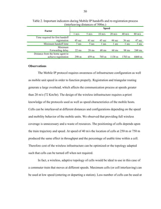
![51
medium speeds (going through construction and semaphore zones). Finally, minimum
cells can be used at high speed (inter-city crossing).
Mobile networking protocols, such as Mobile IP, are not designed to handle high-
speed gracefully. Such protocols produce considerable overhead and high forwarding
delay. We found out that protocols based on registration and non-aware packet re-routing
are not appropriate for speeds higher than 20 m/s.
Re-Examining the Performance of Mobility Protocols using the Columbia Ns-based
Micro-Mobility Suite
The previous subsection presented the experiments and simulations of the Mobile
IP protocol with no optimizations and including the two-ray ground attenuation model for
the entire simulation. Although both scenarios were modeled with ns, the micro-
mobility suite from Columbia assumed the following:
• A simple-distance propagation model replaced the two-ray ground model.
This model allows the base-station to provide connectivity to a certain
node when its location is within a range and zero connectivity when
outside. The two-ray ground model used in the previous results was
overridden. [Widm00]
• Base-upon the simplified propagation model, a new handoff algorithm was
created by characterizing the distance where the mobile node is located
with respect to the base-station, with the denominations of: near range, far
range, and unreachable A mobile node will handoff according to a set of
preference rules depending on the distance of the mobile host and a series
of priorities in the base-stations. [Widm00]
Since new simulative conditions and assumptions are made in the micro-mobility
suite, the Mobile IP simulation was reran and reexamined under the new conditions.
Hence, the same experiments simulated in the previous subsection, including the
performance on throughput and latency for UDP and TCP traces were measured again.](https://image.slidesharecdn.com/hernandezefinal-100909142132-phpapp01/85/Adaptive-Networking-Protocol-for-Rapid-Mobility-64-320.jpg)
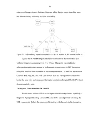
![52
Campbell, et al. [Camp00, Camp01] used a version of ns that included the
assumptions presented above and measured the performance of micro-mobility protocols
for the network topology shown in Figure 21. Although the results presented by
Campbell showed a great improvement on the performance of the protocols: HFA
[Perk96c], Cellular IP [Valk98], and Hawaii [Ramj99]. This chapter reexamines those
results and studies the effects of speed in micro-mobility protocols.
C-host W(0)
0.6.0 0.0.0
W(1) W(2)
0.1.0 0.2.0
W(3) W4) W(5)
0.3.0 0.4.0 0.5.0
Mobile Host 0.7.1
BS(1) BS(2) BS(3) BS(4)
1.0.0 2.0.0 3.0.0 4.00
Figure 21. Infrastructure used for simulations on HAWAII, HFA, and Cellular IP
As shown in Figure 21 a set of intermediate nodes are required in HFA to
minimize the number of updates made to the root node or the Home Agent. Even though
a hierarchy improves the performance during handoff, also increases the number of
intermediate nodes. This increment on the number of resources involves a significant
raise in the cost of the network infrastructure and the number of intermediate nodes on
the network. In order to maintain a consistent experiment with the train scenario as in
Hernandez, et al. [Her01], the architecture on Figure 14 (also Figure 22) was used for the](https://image.slidesharecdn.com/hernandezefinal-100909142132-phpapp01/85/Adaptive-Networking-Protocol-for-Rapid-Mobility-65-320.jpg)
![54
value for UDP in the Mobile IP plot as shown in Figure 29. UDP performance was not
investigated by Campbell et al. but those results are presented in this subsection.
Additionally, all Cellular IP simulations were ran using “semi-soft” handoff, while
the size of the handoff buffer was kept the default value assumed to be 1, although this
parameter is not shown in the simulation code but in the documentation provided by
Columbia [Valk98].
The cell coverage was set to supply a 30 m overlap area and a separation of 500
m between base-stations, as shown in Figure 22, the link delay increments from 10ms to
k×10 ms at the kth base-station as in the model shown in Figure 14.
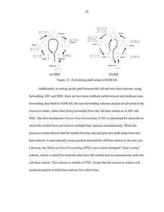
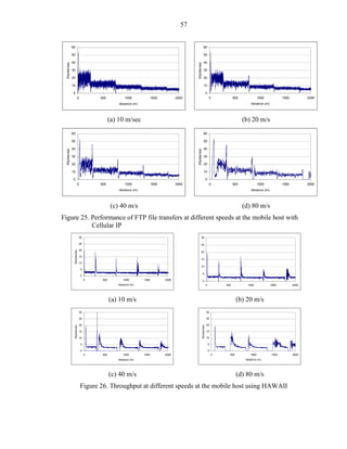
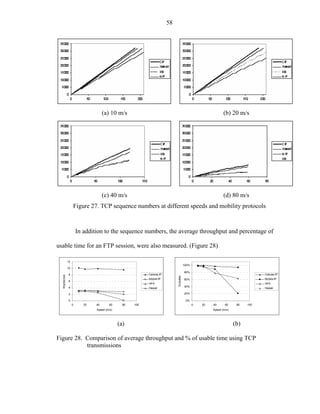
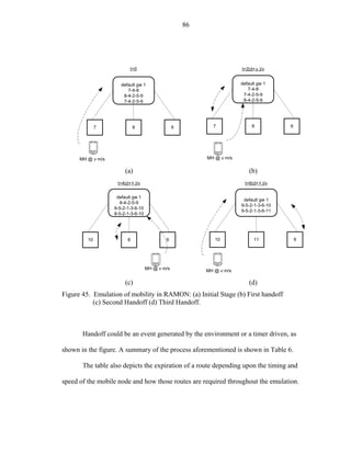
Figure 23 depicts the throughput of TCP transfers measured at the mobile unit. As
expected, the connectivity diminishes as the speed of the mobile host increases.
Although, Figure 23.a and Figure 15.b are the same experiment, the micro-mobility suite
provides a better performance given the simplicity of the model used and the
improvements in the handoff algorithm based upon the simple propagation model.
In fact, connectivity is observed even at 80 m/s when no observations were
captured using a more complex propagation model and without the improved handoff
algorithm based on GPS (Global Positioning System) information available at the mobile
node; however, it’s not clear the mechanism used by Widmer [Wid00] in the creation of
the NOAH (Non Ad-Hoc routing agent)](https://image.slidesharecdn.com/hernandezefinal-100909142132-phpapp01/85/Adaptive-Networking-Protocol-for-Rapid-Mobility-67-320.jpg)
![55
30 30
25 25
20 20
Kbytes/sec
Kbytes/sec
15 15
10 10
5 5
0 0
0 500 1000 1500 2000 0 500 1000 1500 2000
distance (m) distance (m)
(a) 10 m/s (b) 20 m/s
30 30
25 25
20 20
Kbytes/sec
Kbytes/sec
15 15
10 10
5 5
0 0
0 500 1000 1500 2000 0 500 1000 1500 2000
distance (m) distance (m)
(c) 40 m/s (d) 80 m/s
Figure 23. Throughput of Mobile IP with no optimizations and FTP transfers
Therefore the improvement observed when using the micro-mobility suite is
greatly affected by the use of the NOAH agent during the simulations. As shown in the
figures, the performance of Mobile IP diminishes at higher rates of handoff and speeds.
Similarly, Figure 24 shows the performance of Hierarchical Foreign Agents (HFA)
performed as good as the simulated Mobile IP implementation [Hern01]. The hierarchy is
not exploited and the results shown here for HFA represent the worst-case scenario of an
unbalanced tree. The limited regionalization of the location updates reflects only when
the wired network provides a well balanced tree. Even though, this is the worst case
scenario for a hierarchical structure, Figure 24 depicts a better performance at speeds
greater than 40 m/s, which indicates that regionalization and location directory
distribution are key factors on the improvement of Mobile IP.
.](https://image.slidesharecdn.com/hernandezefinal-100909142132-phpapp01/85/Adaptive-Networking-Protocol-for-Rapid-Mobility-68-320.jpg)
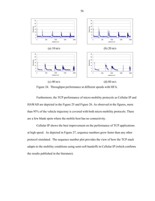
![59
As depicted in the pictures, Cellular IP and HAWAII provide a better connectivity
with almost 100% of usable time, while Mobile IP depicted the worst behavior at 80 m/s.
The performance at 40 m/s averaged the other micro-mobility protocols, which was not
expected. Campbell [Camp02] showed a similar behavior for the micro-mobility
protocols where Hawaii and Cellular IP barely diminishes the throughput at 20
handoff/min.
In Broch [Broc98] and Holland [Holl99] an increase on the average speed of
mobile units results in a much higher reduction of the performance and the average
throughput. In fact, Fladenmuller [Flad99] registered handoff times of at least 2 seconds
on a testbed using WaveLAN cards at 3Mbps. Similar results were explored by [Vat98]
and the effect of DHCP servers and clients in co-located care-of-addresses. Both papers
were consistent with the simulation done with ns and the initial settings used by
Hernandez [Hern01]
Therefore the results shown here with Mobile IP indicate an inconsistency
between implementation for the simulation packages as well as for simulation
assumptions. For instance, Figure 28 shows the percentage of usable time at 40 m/s
shows that 80% of the time Mobile IP provides connectivity, whereas in Figure 16 only a
10% was observed.
The incongruence in the results lead us to conclude that a minor modification on
handoff protocols and simplification of simulative assumptions causes great
improvements on the performance and misleading results. The assumptions made during
the simulations presented by Campbell, et al, [Camp02] and the use of the NOAH agent
augmented the performance numbers.](https://image.slidesharecdn.com/hernandezefinal-100909142132-phpapp01/85/Adaptive-Networking-Protocol-for-Rapid-Mobility-72-320.jpg)
![60
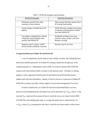
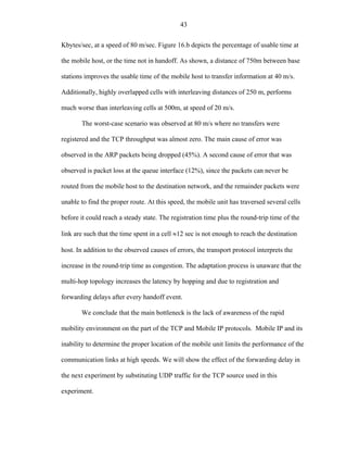
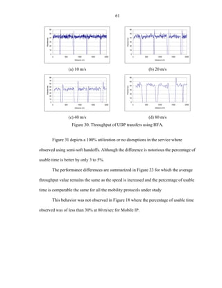
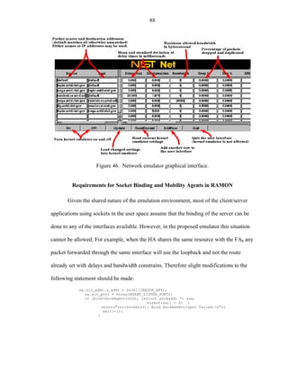
Throughput performance of UDP transmissions
Similar experimentation scenarios were conducted with the UDP protocol using a
Constant Bit Rate flow. However, the results for throughput on UDP transmissions were
not measured in [Camp02]. As shown in the Figure 29, Figure 30, Figure 31 and Figure
32, the micro-mobility protocols provide a minor improvement in the performance of
UDP transmissions on Mobile IP
100 100
90 90
80 80
70 70
Kbytes/sec
Kbytes/sec
60 60
50 50
40 40
30 30
20 20
10 10
0 0
0 500 1000 1500 2000 0 500 1000 1500 2000
distance (m) distance (m)
(a) 10 m/s (b) 20 m/s
100 100
90 90
80 80
70 70
Kbytes/sec
Kbytes/sec
60 60
50 50
40 40
30 30
20 20
10 10
0 0
0 500 1000 1500 2000 0 500 1000 1500 2000
distance (m) distance (m)
(c) 40 m/s (d) 80 m/s
Figure 29. Throughput of UDP transfers using Mobile IP
In fact, at speeds raging from 10 to 40 m/sec, HAWAII, HFA, and Mobile IP
depict very similar performance values of throughput and usable time.](https://image.slidesharecdn.com/hernandezefinal-100909142132-phpapp01/85/Adaptive-Networking-Protocol-for-Rapid-Mobility-73-320.jpg)
![63
60
100%
50
80%
40 Cellular-IP Cellular-IP
Kbytes/sec
% Usable
Mobile-IP 60% Mobile-IP
30
HFA HFA
20 40%
Hawaii Hawaii
10 20%
0 0%
0 20 40 60 80 100 0 20 40 60 80 100
Speed (m/s) Speed (m/s)
(a) (b)
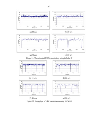
Figure 33. Average UDP throughput and percentage of usable time
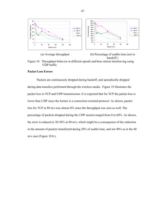
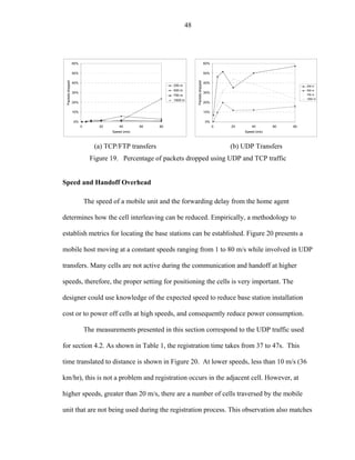
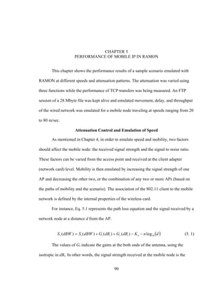
Percentage of error during the simulative experiments
Finally, another parameter measured during the simulations conducted was the
percentage of packets dropped or the error. As expected these values represent the
packets dropped due to UDP flows. There is a great different among the observed results
and the measured by Hernandez, et al. [Hern01]. Figure 19 shows an error value
fluctuating from 0 to 60% indicating also that the percentage of error increases for
Mobile IP with respect to the speed linearly. Improved mechanisms of buffering and
soft-handoff used by Cellular IP and HAWAII, reduced packet loss and indeed better
performance.
Observations
The simulation experiments conducted with the micro-mobility suite showed
inconsistencies with respect to the initial simulation of Mobile IP. The incongruence
result indicates that the implementation decisions made on the simulator as well as the
simulation assumptions used by the developer are not consistent and the results cannot be
fully trusted. For instance, Figure 28 shows the percentage of usable time at 40 m/s was](https://image.slidesharecdn.com/hernandezefinal-100909142132-phpapp01/85/Adaptive-Networking-Protocol-for-Rapid-Mobility-76-320.jpg)
![64
80% for Mobile IP, whereas in Figure 16 only a 10% observed, both simulations were
run using the same topology and physical conditions. We found that the main cause of
error is the utilization of the NOAH agent which augmented the performance numbers
and the results for Mobile IP by using an improved handoff mechanism and the
simplification of the propagation model.
18
16
14
12 CIP
Error (%)
10 MIP
8 Hawaii
6 HFA
4
2
0
0 20 40 60 80 100
Speed (m/s)
Figure 34. Percentage of packets dropped TCP/UDP combined
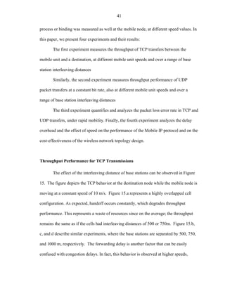
Additionally, Figure 33 indicates a minor diminishment on performance of UDP
with respect to the speed of the vehicle. This fact contradicts other research efforts in
which the throughput value for UDP transfer decreases as speed increases [Broc98,
Holl99, and Hern01] for ad-hoc and infrastructure networks.
Therefore, it is not clear whether or not the micro-mobility protocols performance
measured were outlined in a realistic scenario. This research has concentrated its effort
towards the creation of an emulation/simulation platform, in order to eradicate any
erroneous assumption or overestimation of the mobility protocols in 802.11b-based
networks.](https://image.slidesharecdn.com/hernandezefinal-100909142132-phpapp01/85/Adaptive-Networking-Protocol-for-Rapid-Mobility-77-320.jpg)
![CHAPTER 4
THE RAPID MOBILITY NETWORK EMULATOR
We showed that the performance of mobility protocols greatly depends on
simulative assumptions made by the researcher, which in general affect the out coming
results of the experiments performed. The simplification of environmental parameters
reduces the simulation time as well as the implementation complexity. Realistic testing is
almost never conducted, and many simulation experiments are not replicable. In fact, the
lack of experimentation on real scenarios is a common factor in today’s research.
Pawlikowski, et al. [Paw02] determined that 76% of the authors in IEEE journals of
simulation-based papers were not concerned with the random nature of the results and
many other simulation studies were not replicable. Hence, the excessive use of simulation
tools opens the door for more realistic approaches using network emulation analysis and
experimentation which is easier to replicate.
Emulation also brings several advantages over the simulation approach. Firstly,
applications at different network layers can be tested without special modifications on the
API of the target application by isolating the network and transport layers of the system
as an independent variable. Also, the implementation of network and lower-layer
protocols can be performed in the real scenario without first adjusting the implementation
to the constraints provided by the simulation environment. A very important advantage of
the emulation is found in the complexity of the algorithms and the computation time
required during simulation. For example, a Mobile IP simulation involving 1-mobile unit
66](https://image.slidesharecdn.com/hernandezefinal-100909142132-phpapp01/85/Adaptive-Networking-Protocol-for-Rapid-Mobility-79-320.jpg)
![67
and 20 base-stations generates a 500 Mbytes trace file and more than 3 hrs of processing
on a heavy duty server for a simulation time of 600s. On the contrary an emulation
scenario takes the real-time stipulated in the clock or approximately 600 s.
Our scenario with traveling vehicles at speeds ranging from 0 to 80 m/s (0 to 288
Km/hr), a very costly setting, is not an option for a full emulation environment. Thus, our
idea was define a suite of tools to experiment with existing mobility protocols and study
their behavior in high-speed mobile environments. RAMON combines software and
hardware components to produce realistic conditions and capture the limits of physics in
actual mobile systems. The emulator provides the necessary wireless and wired
infrastructure to allow experimental testing of access-points, network nodes, and antennas
in order to encourage the design of better mobile networking protocols. In RAMON, we
strive to expand the extent to which we use emulation by leveraging on existing
emulation tools.
Many research efforts have been conducted for wired-network emulators. Several
of those are mainly focused to end-to-end network delay emulators for example:
• ENDE [Yeom01]: This emulator created at Texas A&M University,
simulates the internet and end-to-end network delay using ICMP packets
as a real time traffic source.
• ONE [All97]: The Ohio Network Emulator implements an emulator for
transmission, queuing, and propagation delay for two computers
interconnected by a router of a network representation.
• NIST net [NIST01]: The National Institute of Standards and Technology
(NIST) counts with a network emulator that allows an inexpensive PC-
based router to emulate numerous complex performance scenarios,
including: tunable packet delay distributions, congestion and background
loss, bandwidth limitation, and packet reordering / duplication.](https://image.slidesharecdn.com/hernandezefinal-100909142132-phpapp01/85/Adaptive-Networking-Protocol-for-Rapid-Mobility-80-320.jpg)
![69
user to enter the parameters of emulation. Once the necessary parameters are provided,
it’s the emulator’s job to emulate the scenario.
The Architecture
The design of mobile network emulator started with setting up a physical testbed
comprising some embedded computers, the mobility agents, IEEE 802.11b access points,
some networking hubs, attenuation control, and a centralized router. A laptop or a PDA
(iPAQ, Palm) can be used as mobile hosts. The movement of a mobile host is emulated
by following a pattern of attenuation of each access point antenna. Therefore, each access
point was connected to an attenuator, and all the attenuators connected to an attenuation
control unit.
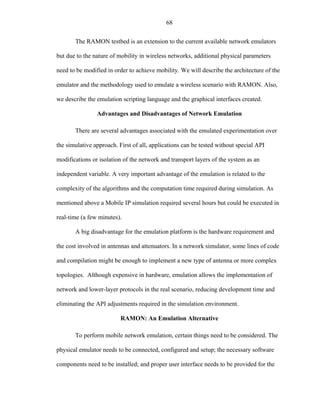
Figure 35 depicts the architecture of RAMON and the emulated infrastructure at
the levels of wireless and wired-networks. As shown in the picture, the emulator uses
three servers for mobility management and routing, each of the servers is loaded with
Linux (RedHat 7.1) as the main operating system. The Linux platform is widely
supported by the routing daemons and mobile protocols such as Cellular IP and Mobile
IP, among many others. [Vlak98, Perk96]
For instance, in case of Mobile IP, the components called HA and FAs can be
easily mapped to the architecture above to Home Agent, Node 1, Node 2, and Node 3.
The figure also depicts the network emulator that represents the wired-infrastructure and
the interconnection of that infrastructure to the Campus network. The wired-network
emulator in the RAMON testbed could be any of the available in the public domain,
ENDE, NIST net, or ONE. However, the NIST net emulator provides a more robust](https://image.slidesharecdn.com/hernandezefinal-100909142132-phpapp01/85/Adaptive-Networking-Protocol-for-Rapid-Mobility-82-320.jpg)
![73
• Location information and emulation of the wired-network infrastructure
used by the wireless network.
• Emulation granularity of intervals of time required by the emulator to
update the position and movement of the mobile node.
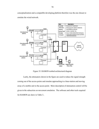
Table 4. Language used by the emulation script
ns script Emulation script Description
$BS X_ $BS name X= Sets the coordinates of the
$BS Y_ $BS name Y= Base-station
set BS [$ns node IP] $BS name IP= Sets an IP Address for the
base-station
set power 0.289 $BS name power=xxx The power level in mW in the
access-point
Set HA… /FA… $HA name IP IP_gate Sets the HA/FA at an IP
$FA name IP1 IP2 IP3 address, it could be the same
as the BS . The FA could use
up to 3 addresses for HFA
implementations.
set Mobile IP 1 $protocol=”MIP“ The protocol being used
set wiredNode [$ns node $IP] $WiredNode name IP1 Creates a Wired Node with
IP2 IP3 three interfaces.
$ns duplex-link $node1 $Link IP1 IP2 bw Creates a Link between two
$node2 $bw $latency latency interfaces using certain
DropTail bandwidth and latency values
$ns at $time [$MH etdest x y $MH time x y speed Sets the destination position
speed] and speed of mobile host.
Acceleration = 0.
$ns at $time start - Starts after it’s called
$ns at $time end $end time End of the emulation
$set opt(prop) $Propagation=”TwoRa Sets the propagation model
Propagation/TwoRayGround yGround”|”PathLoss”|a being used.
ny other.
N/A $granularity X Updates attenuation and speed
every X ms
For instance, a base-station maps an access-point which at the same time is
connected to an attenuator controller. The controller allows the simulation of mobility
and handoff between base-stations. The X and Y values at the base-station with respect
to the original position of the mobile node at (0,0).](https://image.slidesharecdn.com/hernandezefinal-100909142132-phpapp01/85/Adaptive-Networking-Protocol-for-Rapid-Mobility-86-320.jpg)
![74
$BS1 bs1 X = x
$BS1 bs1 Y = y
The creation of a wired node is similar as done in ns, with the exception that in
the emulator script requires of three IP addresses using the 4-byte notation.
TCL ns script Emulator
set WiredNode [$ns node 0.0.0] $WiredNode [$ns node IP1 IP2 IP3]
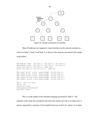
We assume that the wired architectures used for the different simulation occurs
using binary trees and therefore each network node defines three points of access or three
network interfaces.
Additionally, links can be emulated as described by the simulator. For example,
the ns statement $ns duplex-link $WiredNode1 $WiredNode2 10Mb 2ms DropTail
allows the creation of a link between two wired nodes at 10 Mbps with an average delay
of 2 ms. The DropTail queuing model is the only available in the current emulator and
represents a simple FIFO queue with packet drops on overflow. However in the emulator,
instead of using the $WiredNode value, IP addresses should be used to link each other
and create the routes. The syntax used is:
$Link $IP1 $IP2 $bw $latency
Emulation of Speed and Mobility
In order to emulate speed, two factors should affect the mobile node: the received
signal strength and the signal-to-noise ratio. These factors can be varied at the network
card level, and they can emulate mobility by associating the mobile unit to a network
where the signal is automatically controlled.
Signal strength can be varied with the aid of programmable attenuators, an a
simple model of attenuation is describe in (Eq 4.1)](https://image.slidesharecdn.com/hernandezefinal-100909142132-phpapp01/85/Adaptive-Networking-Protocol-for-Rapid-Mobility-87-320.jpg)
![75
2
χ
S r = S t Gt G r (4.1)
4πd
Therefore the attenuation factor at different speeds depend on how the value of d
changes with respect of t, time. In other words, at constant speed v=d/t or v=vot+(at)2/2
for constant acceleration.
The attenuation factor can be then written as shown in (Eq. 4.2), as the value
given by 20 log10(vt). The attenuator has a range from 0 to –127 dB for the JFW
Industries COP3012 [JFW01].
λ
S r (dBW ) = S t (dBW ) + Gt (dBi ) + Gr (dBi ) + 20 log10 − 20 log10 (d ) (4.2)
4π
Given other propagation models, different attenuation equations can be
implemented at the attenuation controller and therefore emulate different environments.
Even more complex models can be combined to improve the mobility conditions at the
emulator.
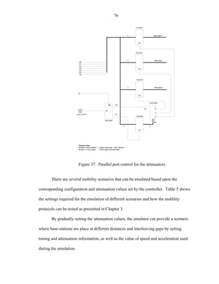
Figure 37 depicts the diagram for the proposed attenuation control and
codification of the values on the Equation 2. The circuit takes D7 from the parallel port to
determine if the value to be written refers to the selected attenuator or the factor of
attenuation used for the simulation. Additionally, attenuation values can be set from any
range and can increase and decrease according to the model implemented in the
controller.](https://image.slidesharecdn.com/hernandezefinal-100909142132-phpapp01/85/Adaptive-Networking-Protocol-for-Rapid-Mobility-88-320.jpg)
![77
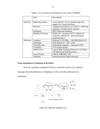
Table 5. Scenarios of mobility for the wireless LAN.
Scenario Attenuator 0 Attenuator 1 Attenuator 2
No connectivity -127 dB -127 dB -127dB
Once cell 0 dB <set < -80 dB -127 dB -127dB
Two overlapped cells 0 dB < set < -80 dB 0 dB < set < - 80 dB -127 dB
Three overlapped cells 0 dB < set < -80 dB 0 dB < set < - 80 dB 0 dB < set < - 80 dB
Mobility protocols, such as IEEE 802.11b, can automatically select a value of
bandwidth of 1,2,5, and 11 Mbps, at a signal strength of –94dBm, -91dBm, -86dBm, and
–82dBm respectively, which in open space represents a distance from the base-station of
550m, 400m, 270m, and 160m, respectively. This information correspond to a standard
Orinoco wireless network card with no external antenna [Ori01]
Similarly, the access point transmitting at 100mW (20dBm) provides a
theoretical attenuation and data rates as shown in from Figure 38, and based upon the
values provided by the manufactured [Cis01]
distance (m)
0 12 distance (m)
0
-10 1 101 201 301 401 501 601
10 0 100 200 300 400 500 600 700 800
-20 PL(d) 100mW
-20
-30 Data rate PL(d) 1mW
Data Rate (Mb/s)
8
Path Loss (dBm)
-40 -40
PL (dBm)
PL(d) (5mW)
-50 6 PL(d) (30mW)
-60
-60
PL(d) 100 mW
4
-70 -80
-80
2
-90 -100
-100 0
-120
(a) Path loss and data rate for Cisco AP- (b) Path loss equations at different
350 transmission power levels (n=2.5)
Figure 38. Data rates and path loss attenuation for CISCO AP-350
Data rates of 11 Mbps can be maintained for 325m from the center for the cell
while dropping to 1Mbps at the extreme of the cell or at approximately 700 m with
100mW of transmission power in open space. As expressed by Equation 4.3, the power
received due to the path loss (PLrecv) is an expression where n is determined empirically](https://image.slidesharecdn.com/hernandezefinal-100909142132-phpapp01/85/Adaptive-Networking-Protocol-for-Rapid-Mobility-90-320.jpg)
![78
as well as P(do) is 40 dB at 2.4GHz. There are several variations to the path loss model or
shadowing model as found in the literature and not covered in detail here [Rapp95]
d
PLrecv = Ptx − P(d o ) − 10n log( ) (4.3)
do
Algorithm for Emulated-Mobility
The semantics of the network emulation scripting language require the use of
network addresses and not only the base-station id. Henceforth, the emulation process is
as follows:
4+3i 5+3i
RAMON initial expires
Node 1 3+3i 5+3i
Node 2 4+3i 3+3(i+1)
Node 1 Node 2 Node 3
Node 3 5+3i 4+3(i+1)
3+3i
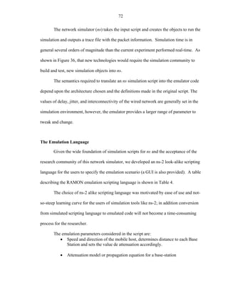
Figure 39. Handoff sequence for emulation
As shown in Figure 39, at the ith handoff, Node 1, Node 2 and Node 3 are required
to represent the element in the network topology. In other words, routes and emulation
of wired lines between the MH and the CH can be initialized and expired accordingly.
The figure indicates that Node 1 requires being available at 3+3i handoffs and routes will
expire at 5+3i number of handoff expected by the MH. A handoff process is known since
the trajectory and range information is provided by the user. Each handoff instance
occurs. The basic emulation process is presented as follows:](https://image.slidesharecdn.com/hernandezefinal-100909142132-phpapp01/85/Adaptive-Networking-Protocol-for-Rapid-Mobility-91-320.jpg)
![79
Emulation(MH, granularity)
1. initializeResources( )
2. DetermineRoutes(route[][], time_end[], trajectory(MH));
3. while timer() > end_simulation
4. do
5. if timer>=timer_end[k]
6. then k++
7. createRoute(route[k][1..3], time_end[k]);
8. expireRoute(route[k-1][1..3])
9. emulateMovement(granularity, MH )
10. return
First determines the routes and the emulation values for the link are calculated
thru the formula BW←MIN(BWk, BSi, BSj) and the Latency ←MAX(latencyk, BSi, BSj),
between two base-stations.
1. emulateMOVEMENT(granularity, MH)
2. MH.x ←granularity×speedx + MH.x
3. MH.y ←granularity×speedy + MH.y
4. attenuator(0, distance(BSi, MH))
5. attenuator(1, distance(BSi+1, MH))
6. attenuator(2, distance(BSi+2, MH))
7. if expiredRoute(i) then i++;
8. return MH
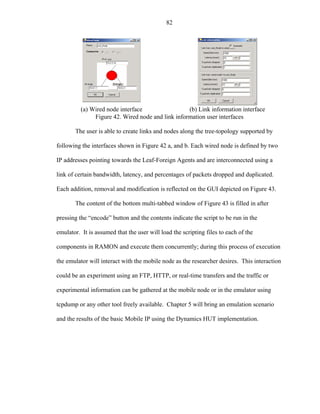
Graphical User Interface for RAMON
In addition to defining the scripting language presented in Table 4, the
proliferation of windows based-computers and the codification process from the
emulation script into the real code and parameters used within the emulator required the
creation of a Computer Aided Software Engineering (CASE) tool. As depicted in Figure
40, the user is able to create a script as described earlier or design the emulated
architecture with the aid of some more user-friendly dialog boxes.
.](https://image.slidesharecdn.com/hernandezefinal-100909142132-phpapp01/85/Adaptive-Networking-Protocol-for-Rapid-Mobility-92-320.jpg)
![80
Figure 40. Graphical user interface for RAMON - CASE tool
Both, the Graphical User Interface (GUI) and scripting-based creation of
emulation scenarios are supported. The GUI will allow a much better visualization for the
emulated networks and protocols to test in the emulation platform. Previous work in the
Harris Networking and Communications Laboratory at the University of Florida has been
conducted towards the creation of ns scripts aided with a GUI, this work is called
CADHOC [Shah01] which is a tool targeted to investigate ad-hoc networks.
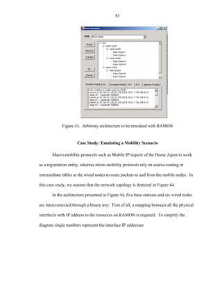
Figure 41 depict the options and generated scripts to be placed in each of the
entities of RAMON. The user is able to add a root node, a wired node, or a base station.
The topologies that are currently supported by RAMON are any variation of a binary tree
for the wired nodes, and any combination of slightly overlapped base stations. In other
words, the base stations cannot be overlapped and should be geographically located
according to the timing restrictions shown in Figure 39 for a proper emulation of the](https://image.slidesharecdn.com/hernandezefinal-100909142132-phpapp01/85/Adaptive-Networking-Protocol-for-Rapid-Mobility-93-320.jpg)
![81
scenario. The application was created using the newly available .NET platform and the
C# programming language from Microsoft, Corp [Conr00, Gun01].
Figure 41. GUI for the architecture to emulate and the scripting contents of each
element in RAMON
This platform allows a fast deployment of the current emulation interface and the
proper dissemination of the use of the rapid mobile emulator on the internet, as part of a
remote experimentation project.](https://image.slidesharecdn.com/hernandezefinal-100909142132-phpapp01/85/Adaptive-Networking-Protocol-for-Rapid-Mobility-94-320.jpg)
![87
The Linux service route and cnistnet [NIST01] can be used to create the routes, as
well, as the creation of the emulation of the links. For route creation an example for a HA
routing the network 192.168.2.0 thru the interface 1.2 would be:
$route add –net 192.168.2.0 netmask 255.255.255.0 dev eth1:0
Table 6. Routing table configuration throughout the emulation process
RAMON element Starts Expires Network/host Route
Node 1 0 4(d+ε)/v 7 default gw 4
4(d+ε)/v ∞ 10 default gw 6
Node 2 2(d+ε)/v 4(d+ε)/v 8 default gw 4
6(D+ε)/V ∞ 11 default gw 6
NODE 3 0 ∞ 9 default gw 5
NETWORK 0 2(d+ε)/v 1,2,4,5 default gw 1
EMULATOR 7-4-8
7-4-2-5-8
7-4-2-5-9
2(d+ε)/v 4(d+ε)/v 1,2,3,4,5,6 default gw 1
7-4-8
7-4-2-5-9
8-4-2-5-9
4(d+ε)/v 6(d+ε)/v 1,2,3,4,5,6 default gw 1
8-4-2-5-9
8-5-2-1-3-6-10
9-6-2-1-3-6-10
6(d+ε)/v ∞ 1,2,3,5,6 default gw 1
9-5-2-1-3-6-10
9-5-2-1-3-6-11
10-6-11
Similarly the point-to-point links are configuring with the netmask
255.255.255.255. While route provides the proper routing information, the bandwidth
and link emulation is done with cnistnet as follows:
$cnistnet –a 192.168.2.0 192.168.1.2 --delay 2 –bandwidth 10](https://image.slidesharecdn.com/hernandezefinal-100909142132-phpapp01/85/Adaptive-Networking-Protocol-for-Rapid-Mobility-100-320.jpg)
![89
The underlined piece of code should be changed to the specific IP address
configured at the specific interface. In other words:
lip = ipt->table[ip_cnt].dwAddr;
lnp = ipt->table[ip_cnt].dwMask;
sa->sin_addr.s_addr = lip & lnp | ~lnp;
By doing so the HA will only listen to the IP address specified and not to any
interface. The Mobile IP implementation we have chosen that fulfills these requirements
is the Helsinki University of Technology (HUT) which is called Dynamics [Fors99a,
Fors99b]](https://image.slidesharecdn.com/hernandezefinal-100909142132-phpapp01/85/Adaptive-Networking-Protocol-for-Rapid-Mobility-102-320.jpg)
![91
summation of all the gains (St, Gi) minus the propagation loss due to fading of the signal.
This propagation loss depends on the many characteristics of the terrain and was
empirically defined by [Pahl95] using different values of Ko and n, depending upon
different terrain conditions at different frequency values.
Propagation Model
The experimental values and equations used for the propagation in RAMON
correspond to the modeling for indoor and micro-cellular environments [Pahl95], which
is depicted by Eq 5.2. The empirical model indicates that the attenuation is negligible at
closer distance from the antenna, and quickly logarithmically decays at certain distances
using different values of n and Ko, In this case 10, and 20 are used in Eq. 5.2.
0, d ≤ R / 100 d >= 1.2 R
(5.2)
A(d ) = 10 + n log( d ), R / 100 < d ≤ 0.9 R
20 + 10(n + 1.3) log(d ), d > 0 .9 R
In Eq 5.2, d is the distance between the AP and the mobile node and R is the cell
ratio (which has a value of 500 m). Also we used a simple square attenuation model,
which is used to simplify and determine the handoff rate.
0 0 ≤ d ≤ 0.9 R
A(d ) = (5.3)
128 d > 0.9 R
Although, the models depicted several values of attenuation to use in the
attenuator, experimental measurements indicated that the valid range of attenuation was
from 0 to 60 dB, approximately. Anything bellow this value was affected by the AP
signal leakage, which is difficult to completely circumvent.](https://image.slidesharecdn.com/hernandezefinal-100909142132-phpapp01/85/Adaptive-Networking-Protocol-for-Rapid-Mobility-104-320.jpg)
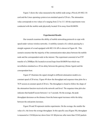
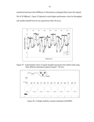
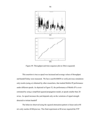
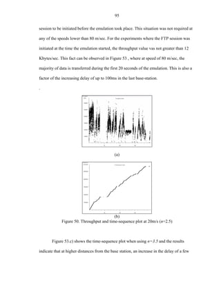
![96
hundred of milliseconds is enough to drop the bandwidth to almost zero after 30 seconds
of emulation
Other test bed platforms and experimental results have related the handoff rate as
physical variable that is equivalent to speed, which is correct for a simple attenuation
model (Eq.5.3). Campbell, et al. [Camp01] presents the throughput as a function of the
handoff rate between two access points only, without considering signal strength effect or
any of the variable conditions included in RAMON, (e.g., increased delay on crossing
different access points, different attenuation models, realistic Mobile IP implementation,
among others). The results shown in this paper indicate that simply forcing handover
between two access points at different rates is not sufficient to demonstrate the effects of
speed on mobile protocols.
Figure 52 depicts the difference on average throughput and speed using different
attenuation models. The figure shows a great level of degradation on the average value of
throughput as speed increased of at least 50% at 80 m/sec when compared to the average
throughput at 20 m/sec. This expected performance loss is greater than the expected by
Campbell [Camp01] of only 25% at 20 handoff/min or an equivalent speed value of 300
m/sec. (assuming a cell diameter of 1000 m) Lastly, we can assure that the effectiveness
of a handoff protocol needs to be thoroughly tested using emulated conditions that
resemble realistic scenarios. Therefore, in order to cope with the variability of signal
strength, network latency, and speed, an emulation environment as RAMON is very
much needed for the testing of mobile and wireless networks.](https://image.slidesharecdn.com/hernandezefinal-100909142132-phpapp01/85/Adaptive-Networking-Protocol-for-Rapid-Mobility-109-320.jpg)
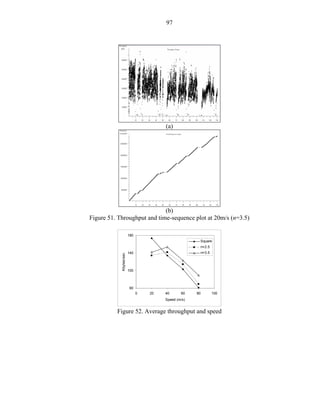
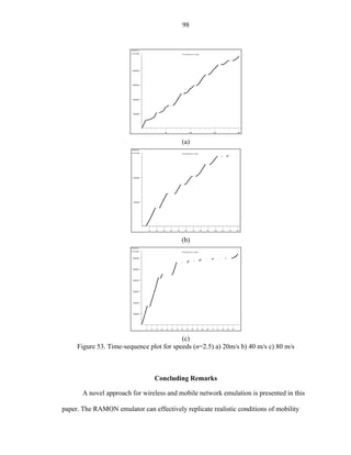
![99
providing interesting insights and observations previously unknown and non-observed in
pure simulation experiments such as ns [Hern01]. Using RAMON, we have shown that
handoff and throughput change significantly with the attenuation model used in the study.
Therefore, a careful selection and capture of such models are necessary for obtaining
accurate data about the performance of a given wireless network.](https://image.slidesharecdn.com/hernandezefinal-100909142132-phpapp01/85/Adaptive-Networking-Protocol-for-Rapid-Mobility-112-320.jpg)
![CHAPTER 6
PREDICTIVE MOBILITY AND EXTENSIONS FOR MOBILE IP
As shown in previous chapters, registration and forwarding delay diminishes the
performance of mobility protocols during the updating process of the location directory at
the Home Agent or the hierarchy of foreign agents. In general, the creation of the
respective tunnels, the initialization of new bindings, and forwarding the data directed to
the mobile node are conducted in nonnegligible amount of time. The reactive Mobile IP
mechanisms scheme is unable to respond quickly enough to support rapid mobile
environments. This chapter introduces the predictable framework and the creation of two
new entities that extend the current Mobile IP implementation.
Performance Bottlenecks for Mobile IP
In the majority of mobile networking protocols, the mobile node requires of
registration in order to maintain the home network aware of its mobility, the Home
Location Register (HLR) and the home agent structure used in Mobile IP [Perk96b] are
well known examples of mobile protocols. Hierarchical implementations of Mobile IP
[Fors99] ,such as the Dynamics Mobile IP, required of less initialization time than in non-
hierarchical implementations, although faster, tunnel initialization, binding updating and
handoff management takes a few seconds. Several experiments were conducted in
RAMON and using an agent advertisement time of 1 sec, with no agent solicitation
messages, handoff required approximately 2 to 10 seconds depending upon the speed of
the mobile host as depicted in Chapter 5.
100](https://image.slidesharecdn.com/hernandezefinal-100909142132-phpapp01/85/Adaptive-Networking-Protocol-for-Rapid-Mobility-113-320.jpg)
![101
In a rapid mobility, nonassisted and reactive handoff time is closed in magnitude
to the dwell time in the cell. In order to minimize this factor the mobile protocol should
be able to be preemptive and predict potential locations where the rapid mobile units are
about to cross and handoff will occur faster while maintaining connectivity even at high
speed. In general the inequality presented in Eq. 6.0 illustrates the scenario where the
Mobile IP actually works, although for scenarios where a cell size ranges between 500 to
1000 m. and the mobile unit travels at a speed of 80 m/s, the Tdwell time would be between
6 to 12 seconds, therefore any significant reduction on the handoff time and the
forwarding delays associated with the reactive approach taken by Mobile IP protocol will
allow a better utilization time of the cell.
Tdwell + Thandoff + ε >> T forward + Tregistration + δ (6.0)
The Mobile IP implementation used in RAMON assumes a hierarchy of foreign
agents and follows the majority of recommendations found in drafts for low-latency
handoff in Mobile IP [Elka01] and their own criteria for handoff management [Fors99a].
The Dynamics - HUT Mobile IP system, developed at Helsinki University of Technology
(HUT), is a hierarchical Mobile IPv4 solution for the Linux operating system. The
software consists of three independent daemon executables: Home Agent (HA), Foreign
Agent (FA) and Mobile Node (MN). Figure 54 shows the mechanism followed by the
default configuration of the protocol.. First the mobile node will receive an agent
advertisement message which is created by the FA and broadcasted using ICMP (Internet
Control Messaging Protocol). The advertisement message includes the default route as
well as the correspondent care-of-address of the mobile node. The Mobile Node receives
all the advertisement messages and determines which foreign agents are in its](https://image.slidesharecdn.com/hernandezefinal-100909142132-phpapp01/85/Adaptive-Networking-Protocol-for-Rapid-Mobility-114-320.jpg)
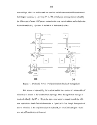
![103
The “Ghost” Entities
The Mobile IP reactive mechanism for handoff is not suitable for rapid-mobility.
We propose two new entities targeted to speed up handoff and improve the performance
of the hierarchical and non-hierarchical implementations of Mobile IP. Our proposals are:
• Ghost Mobile-Node (g-MN) moves with the MN along the different cells
and follows a determined trajectory. The g-MN is a “virtual” repeater
capable of registering and allocating resources in a predictive matter. The
g-MN speeds up handoff and augments the performance of Mobile IP.
The g-MN is cable of replicating the registration request, handling the
creation of the tunnel, and replicating Authentication and Authorization
information from the MN and act on behalf of the MN before is in the
range of the new FA.
• Ghost Foreign Agent (g-FA) is an entity that receives a delegation of
authority from the FA. The g-FA is created in the neighborhood of the
FA. Its main role is to advertise the FA presence from a neighbor FA.
Figure 55.a. shows how a g-FA acts on behalf of LFA2 (Leaf Foreign Agent), so
any MN can include that FA as a potential place for handoff when in LFA1 range. Once
the MN has moved to the vicinity of LFA2 (coming from LFA1), registrations has
already been done and resources have been allocated for the MN. Additionally, the g-FA
has updated the information of available FAs in the MN and handoff decisions can be
taken quicker. Another useful feature of the g-MN is the possibility of buffer all the
traffic coming from the Correspondent Host (CH) towards the MN during the handoff
process. This feature was not implemented in the current proposal for the g-MN and g-
FA.
The goal of the duality (g-MN and g-FA) is very similar to the middleware used
in I-TCP [Bala95, Bala96] or the separation of the wired and the wireless
communication. The interaction performed by the duality (g-MN and g-FA) allocates](https://image.slidesharecdn.com/hernandezefinal-100909142132-phpapp01/85/Adaptive-Networking-Protocol-for-Rapid-Mobility-116-320.jpg)
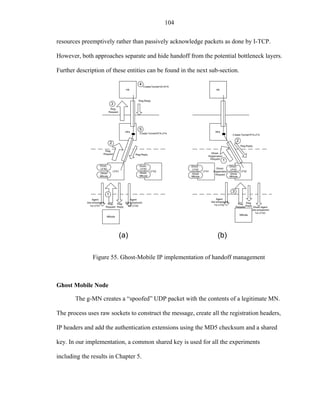
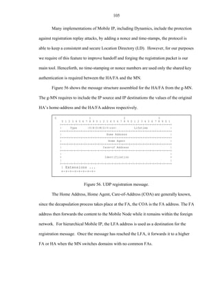
![106
Our implementation allows the use of any MN, while the code for the MN
remains untouched. During the absence of a g-MN, the MN falls back to the reactive
mechanisms of the Mobile IP. The algorithm used by the g-MN is the following:
g-MN (Home Address, HomeAgentAddress)
1. while (true) do
2. FA ←FindClosestFA(MN)
3.. if distance(FA, MN) within threshold then
4. HFA ←FindHighestFA(FA, HomeAgentAddress)
5. Register(FA, Home Address, HFA)
6. end
We assumed that a Global Positioning System (GPS) is on board of the MN. A
substitute for GPS could be any other mechanism to triangulate the position of the MN
based-upon signal strength or thru the use of wireless sensors. .
Other researchers have also determined the importance of GPS in Mobile IP and
routing protocols. A GPS and Mobile IP study was developed by Ergen [Erge02]. Ergen,
et al. indicates that the Advanced Traveler Information Systems (ATIS) are becoming a
popular tool for different transportation authorities around the United States. Los Angeles
and Seattle have deployed sensors and GPS equipped mobile vehicles to predict traffic,
avoid congestion, and maximize the utilization of roads and highways. Ergen reported
that the usage of GPS eliminates the packet loss during handoff and time interval between
packets is good enough to guarantee real-time data delivery.
The g-MN algorithm requires of advanced knowledge of the distance in between
the MN and FAs, similarly to Ergen’s we used the location information to improve
handoff management. Our approach, instead of reacting to the coordinate location,
predicatively determines the distance to the following FA. The g-MN has already access](https://image.slidesharecdn.com/hernandezefinal-100909142132-phpapp01/85/Adaptive-Networking-Protocol-for-Rapid-Mobility-119-320.jpg)
![107
to the foreign network and resource allocation can take place before the arrival of the
mobile node..
The messages created by the g-MN coexist with the MN registration mechanics.
Given the accuracy of the Kalman Filter and the dynamics of vehicular technology
higher-speeds does not allow sudden changes of direction. Therefore, as the vehicle’s
speed increases less the chances for random directions to be taken.
An unresolved problem in our approach is the potential inconsistencies between
the location being updated and the resource allocated. Chances are that two registration
messages will point to two different HFA and two tunnels will be created. Tunnel
creation and packet forwarding took several seconds to be initialized; therefore pre-
registration process is less harmful than non-registering a-priori. The disadvantage is
waste of resources. A registration message issued to the HFA or HA would take a few
milliseconds to arrive and be processed. Therefore, an inaccurate registration will
diminish the overall performance. Full incorporation and awareness is required at the
Home Agent level in order to minimize the effect of g-MN erroneous registration.
Ghost Foreign Agent
Each FA creates g-FA instances at the vicinity of FAs. The g-FA works as if the
signal strength of a certain FA was increased and the coverage area was “augmented” by
a certain factor. In fact, the approach taken by the g-FA is to increment the amount of
resources available. This virtual expansion of resources is very similar to Levine’s
proposal of “shadow clusters” [Levi95]. In shadow clusters, the mobile nodes inform the
base-stations about their location, trajectory and any other parameter required to allocate](https://image.slidesharecdn.com/hernandezefinal-100909142132-phpapp01/85/Adaptive-Networking-Protocol-for-Rapid-Mobility-120-320.jpg)
![108
resources in wireless-ATM networks using micro- and nano-cellular infrastructures. The
algorithm used by the g-FA is presented as follows:
g-FA(ForeignAgent)
1. For each FA in Topology
2. if (distance(FA, ForeignAgent)>threshold) and (FA!=ForeignAgent)
3. SendGhostAgentAdv(ForeignAgent, FA)
4. end
0 1 2 3
0 1 2 3 4 5 6 7 8 9 0 1 2 3 4 5 6 7 8 9 0 1 2 3 4 5 6 7 8 9 0 1
+-+-+-+-+-+-+-+-+-+-+-+-+-+-+-+-+-+-+-+-+-+-+-+-+-+-+-+-+-+-+-+-+
| Type | Length | Sequence Number |
+-+-+-+-+-+-+-+-+-+-+-+-+-+-+-+-+-+-+-+-+-+-+-+-+-+-+-+-+-+-+-+-+
| Registration Lifetime |R|B|H|F|M|G|V| reserved |
+-+-+-+-+-+-+-+-+-+-+-+-+-+-+-+-+-+-+-+-+-+-+-+-+-+-+-+-+-+-+-+-+
| zero or more Care-of Addresses |
| ... |
Figure 57. Agent advertisement message in Mobile IP
The g-FA determines all the FA within a ratio (threshold) and creates an ICMP
packet with the information provided in Figure 57. The care-of-addresses is already a
persistent part of the FA configuration file and sequence numbers can be easily spoofed.
Additionally, the g-FA should assembly the raw socket using the FA address as a source
with a broadcast address as destination.
Location Tracking with the Kalman Filter
The Kalman filter is used to determine the amount of time before the g-MN can
send a registration message and act on behalf of the real mobile node.
Kalman filters have been used in numerous applications ranging from location
tracking and control of physical variables; wireless protocols are not the exception.
D. Dailey, et al... [Dail00] solves the problem of tracking a vehicle and the time to arrival](https://image.slidesharecdn.com/hernandezefinal-100909142132-phpapp01/85/Adaptive-Networking-Protocol-for-Rapid-Mobility-121-320.jpg)
![109
to a certain destination using the Kalman filter. The prediction done by the predictor is
used to inform bus riders and anyone with a smart phone the waiting time of a bus route
in Seattle, WA.
The Kalman filter [Welc02] addresses the problem of trying to estimate the state:
x ∈ Rn of a discrete-time controlled process that is governed by a linear stochastic
difference equation. In general the process is composed of the state (Eq 6.1) and the
measurement vectors. (Eq 6.2)
The Kalman filter assumes that there is a state vector x such that:
x k = Ax k −1 + Bu k + wk −1 (6.1)
with a measurement vector z ∈ Rn such that::
z k = Hx k + v k (6.2)
The equations also include the values of wk and vk are random variables
representing the process noise of the measurement and state vectors. The matrices A,
B, and H relate the states and the dynamics of the system under study. In the Mobile IP
ghost-MN it will represent the velocity and position of the MN at any given time.
In fact, Eq 6.3 shows the relationship of the state vector and the basic dynamics of
the Mobile Node and the well known relationship of a 2-D object moving at constant
speed.
x 1 0 t 0 x wx
y 0 1 0 t y w y
v = 0 + s
0 1 0 v x wx
(6.3)
x s
v 0 0 0 1 v y w y
y ](https://image.slidesharecdn.com/hernandezefinal-100909142132-phpapp01/85/Adaptive-Networking-Protocol-for-Rapid-Mobility-122-320.jpg)
![110
The measurement vector zk = [x y]T is required to determine and use the
FindClosestFA() function in the g-MN algorithm, and is also required in the recursive
mechanics of the Kalman Filter. The filter uses an ongoing cycle which require of the
time-update equations to determine the state ahead of time and the measurement update
which is used to adjust the internal parameters of the filter. With these variables we pose
the problem as a linear Kalman Filter equation:
X k = AX k −1 + wk (6.4)
Z k = Hz k + v k (6.5)
where,
1 0 t 0 wx
0 1 0 t 1 0 0 0 vs wy
A= : H = 0 1 0 0
vk =
v wk = s (6.6)
0 0 1 0 y w
x
0 0 0 1 ws
y
The time-update equations for the Kalman Filter are presented bellow:
x k = Ax k −1 + Bu k + wk −1 (6.7)
Pk = APk −1 A + Q
T
(6.8)
In our scenario B=0 and Pk is the covariance matrix which is estimated from time
step k-1 to step k. The matrix Q = E{wk wkT }.
For the measurement-update equations, the first equation (Eq 6.9) computes the
Kalman gain, Kk, the second equation (Eq 6.10) calculates the value of xk which is used in
Eq 6.7 to compute the predicted value of the state vector. The third equation (Eq 6.11)
updates the covariance matrix Pk.. The value of the co-variance matrix R=E{vk vkT] is
required and in general is the easier to determine since we know already how to measure
the position vector and we can easily dedicate some samples to determine the co-variance
of vk.](https://image.slidesharecdn.com/hernandezefinal-100909142132-phpapp01/85/Adaptive-Networking-Protocol-for-Rapid-Mobility-123-320.jpg)
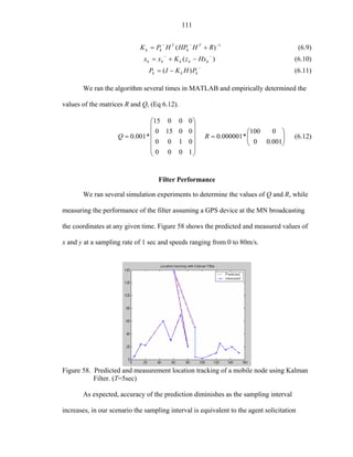
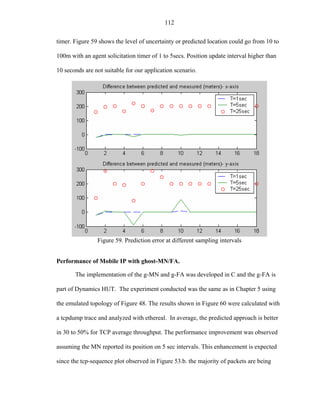
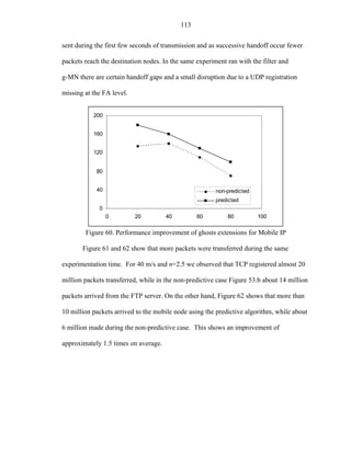
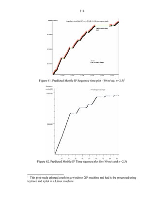
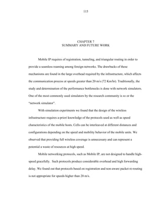
![116
Additionally, we analyzed the micro-mobility protocols, HAWAII and Cellular
IP, both showed significant improvement in the simulator. However, the comparisons
made with Mobile IP under similar assumptions and simulation variables showed a
discrepancy with previous results and observations done with the more restrictive handoff
mechanisms as well as attenuation models.
Since experimentation based-upon simulation software largely depends on the
assumptions and problem constraints, we decided to create an emulation platform tailored
to mimic a more realistic environment of rapidly moving nodes. The emulator, called
RAMON, effectively replicates realistic conditions of mobility providing interesting
insights and observations previously unknown and non-observed in simulation-based
experiments [Hern01].
Handoff is stimulated with the aid of attenuators interacting with the signal
strength of the base-stations and the experimenter can interchange different attenuation
models. Additionally, latency and throughput are also modified in the emulated scenario.
The emulation language provides the abstraction to define the emulated scenario, and a
Graphical User Interface facilitates the schematic representation and graphical
visualization of the wired and wireless topology to be emulated.
Using RAMON, we have shown that handoff and throughput change significantly
with the attenuation model used in the study. Therefore, a careful selection and capture of
such models are necessary for obtaining accurate data about the performance of a given
wireless network. RAMON indicated that highest performance bottleneck is found in the
creation of the tunnel and](https://image.slidesharecdn.com/hernandezefinal-100909142132-phpapp01/85/Adaptive-Networking-Protocol-for-Rapid-Mobility-129-320.jpg)
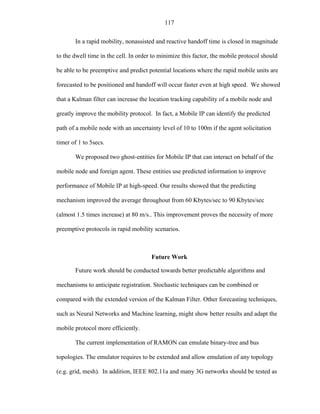
![118
extensions for RAMON. RAMON presented several signal leakage problems which
might require of special covers or cables to reduce signal loss.
RAMON needs improvements in the graphical interface and integration of
visualization tools for throughput, latency, and sequence-time plots.
For long emulation intervals of time, RAMON will required better process
synchronization using logical clocks or the Network Time Protocol (NTP). The
inclusion of realistic GPS systems and emulated noise generation would recreate more
realistic scenarios.
Finally, other protocols could benefit from the g-MN such as the Interlayer Layer
Collaboration Protocol (ILC-TCP) [Chin02] which interacts with the lower layers of the
stack to “freeze” TCP and acquired awareness of the wireless conditions.
Mobile IP version 6 should be investigated with RAMON and predictable
protocols could be investigated further.](https://image.slidesharecdn.com/hernandezefinal-100909142132-phpapp01/85/Adaptive-Networking-Protocol-for-Rapid-Mobility-131-320.jpg)
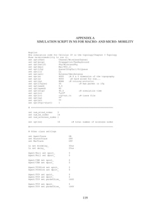
![120
Queue/DropTail/PriQueue set Prefer_Routing_Protocols 1
# unity gain, omni-directional antennas
# set up the antennas to be centered in the node and 1.5 meters above it
Antenna/OmniAntenna set X_ 0
Antenna/OmniAntenna set Y_ 0
Antenna/OmniAntenna set Z_ 1.5
Antenna/OmniAntenna set Gt_ 0.2
Antenna/OmniAntenna set Gr_ 0.2
# Initialize the SharedMedia interface with parameters to make
# it work like the 914MHz Lucent WaveLAN DSSS radio interface
Phy/WirelessPhy set CPThresh_ 10.0
Phy/WirelessPhy set CSThresh_ 1.559e-11
Phy/WirelessPhy set RXThresh_ 3.652e-10
Phy/WirelessPhy set Rb_ 2*1e6
Phy/WirelessPhy set freq_ 914e+6
Phy/WirelessPhy set L_ 1.0
# ==================================================================
source ../lib/ns-wireless-mip.tcl
source cipInit.tcl
Phy/WirelessPhy set Pt_ 0.002822
# intial setup - set addressing to hierarchical
set ns [new Simulator]
$ns color $cipfid($CIP_DATA) blue
$ns color $cipfid($CIP_PAGING) magenta
$ns color $cipfid($CIP_PAGE) orange
$ns color $cipfid($CIP_ROUTE) red
$ns set-address-format hierarchical
# set mobileIP flag; CIP still use some function of MIP
Simulator set mobile_ip_ 1
set namtrace [open /dev/null w]
$ns namtrace-all $namtrace
set trace [open cip-tcp.tr w ]
$ns trace-all $trace
set f1 [open throughput_cip$opt(speed).txt w]
AddrParams set domain_num_ 16
lappend cluster_num 3 1 1 1 1 1 1 1 1 1 1 1 1 1 1 1
AddrParams set cluster_num_ $cluster_num
lappend cluster_num 3 1 1 1 1 1 1 1 1 1 1 1 1 1 1 1
AddrParams set cluster_num_ $cluster_num
lappend eilastlevel 1 1 1 14 1 1 1 1 1 1 1 1 1 1 1 1 1 1
AddrParams set nodes_num_ $eilastlevel
## setup the wired nodes
set W(0) [$ns node 0.0.0]
set W(1) [$ns node 0.1.0]
## create corresponding host
set CH [$ns node 0.2.0]
## create common objects reqd for wireless sim.
if { $opt(x) == 0 || $opt(y) == 0 } {
puts "No X-Y boundary values given for wireless topologyn"
}
set chan [new $opt(chan)]
set prop [new $opt(prop)]
set topo [new Topography]
set tracefd [open "cip-tcpudp"+$opt(speed)+"in" w]](https://image.slidesharecdn.com/hernandezefinal-100909142132-phpapp01/85/Adaptive-Networking-Protocol-for-Rapid-Mobility-133-320.jpg)
![121
# setup topography and propagation model
$topo load_flatgrid $opt(x) $opt(y)
$prop topography $topo
# Create God
create-god $opt(nn)
$ns node-config -mobileIP ON
-adhocRouting NOAH
-llType LL
-macType Mac/802_11
-ifqType Queue/DropTail/PriQueue
-ifqLen 50
-antType Antenna/OmniAntenna
-propType Propagation/TwoRayGround
-phyType Phy/WirelessPhy
-channelType Channel/WirelessChannel
-topoInstance $topo
-wiredRouting ON
-agentTrace ON
-routerTrace OFF
-macTrace ON
# Set tranmission Power so that overlapping area is desired
# Overlapping region between base stations
set overlap 30
set coverage [CellCoverage 1 1 500 500 $overlap]
Phy/WirelessPhy set Pt_ [SetPt $coverage]
set power [Phy/WirelessPhy set Pt_]
set power [Phy/WirelessPhy set Pt_]
## setup Base Station nodes
# Base Station 1
$ns node-config -rxPower $power -txPower $power
set BS1 [$ns node 1.0.0]
[$BS1 set regagent_] priority 1
# Mobile Host
$ns node-config -wiredRouting OFF
$ns node-config -rxPower $power -txPower $power
set MH [$ns node 1.0.2]
$MH MakeMobile
$MH create-watchdog $W(0); # W(0) is GateWay node
$MH set cur_bs_node 0
# enable semisoft handoff
# $MH enable-semisoft
$ns node-config -wiredRouting ON
# Base Station 2
$ns node-config -rxPower $power -txPower $power
set BS2 [$ns node 2.0.0]
# Base Station 3
$ns node-config -rxPower $power -txPower $power
set BS3 [$ns node 3.0.0]
# Base Station 4
$ns node-config -rxPower $power -txPower $power
set BS4 [$ns node 4.0.0]
# Base Station 5
$ns node-config -rxPower $power -txPower $power
set BS5 [$ns node 5.0.0]
# Base Station 6
$ns node-config -rxPower $power -txPower $power](https://image.slidesharecdn.com/hernandezefinal-100909142132-phpapp01/85/Adaptive-Networking-Protocol-for-Rapid-Mobility-134-320.jpg)
![122
set BS6 [$ns node 6.0.0]
# Base Station 7
$ns node-config -rxPower $power -txPower $power
set BS7 [$ns node 7.0.0]
# Base Station 8
$ns node-config -rxPower $power -txPower $power
set BS8 [$ns node 8.0.0]
# Base Station 9
# Base Station 9
$ns node-config -rxPower $power -txPower $power
set BS9 [$ns node 9.0.0]
# Base Station 10
$ns node-config -rxPower $power -txPower $power
set BS10 [$ns node 10.0.0]
# Base Station 11
$ns node-config -rxPower $power -txPower $power
set BS11 [$ns node 11.0.0]
# Base Station 12
$ns node-config -rxPower $power -txPower $power
set BS12 [$ns node 12.0.0]
# Base Station 13
$ns node-config -rxPower $power -txPower $power
set BS13 [$ns node 13.0.0]
# Base Station 14
$ns node-config -rxPower $power -txPower $power
set BS14 [$ns node 14.0.0]
$BS1 set-base $BS1 [AddrParams set-hieraddr [$BS1 node-addr]]
$BS2 set-base $BS2 [AddrParams set-hieraddr [$BS2 node-addr]]
$BS3 set-base $BS3 [AddrParams set-hieraddr [$BS3 node-addr]]
$BS4 set-base $BS4 [AddrParams set-hieraddr [$BS4 node-addr]]
$BS5 set-base $BS5 [AddrParams set-hieraddr [$BS5 node-addr]]
$BS6 set-base $BS6 [AddrParams set-hieraddr [$BS6 node-addr]]
$BS7 set-base $BS7 [AddrParams set-hieraddr [$BS7 node-addr]]
$BS8 set-base $BS8 [AddrParams set-hieraddr [$BS8 node-addr]]
$BS9 set-base $BS9 [AddrParams set-hieraddr [$BS9 node-addr]]
$BS10 set-base $BS10 [AddrParams set-hieraddr [$BS10 node-addr]]
$BS11 set-base $BS11 [AddrParams set-hieraddr [$BS11 node-addr]]
$BS12 set-base $BS12 [AddrParams set-hieraddr [$BS12 node-addr]]
$BS13 set-base $BS13 [AddrParams set-hieraddr [$BS13 node-addr]]
$BS14 set-base $BS14 [AddrParams set-hieraddr [$BS14 node-addr]]
$ns at 0.0 "$CH label Corresponding_Host"
$ns at 0.0 "$W(0) label GateWay"
$ns at 0.0 "$W(1) label CIP_Node"
$ns at 0.0 "$BS1 label BS1"
$ns at 0.0 "$BS2 label BS2"
$ns at 0.0 "$BS3 label BS3"
$ns at 0.0 "$BS4 label BS4"
$ns at 0.0 "$BS5 label BS5"
$ns at 0.0 "$BS6 label BS6"
$ns at 0.0 "$BS7 label BS7"
$ns at 0.0 "$BS8 label BS8"
$ns at 0.0 "$BS7 label BS7"
$ns at 0.0 "$BS8 label BS8"
$ns at 0.0 "$BS9 label BS9"
$ns at 0.0 "$BS10 label BS10"
$ns at 0.0 "$BS11 label BS11"
$ns at 0.0 "$BS12 label BS12"
$ns at 0.0 "$BS13 label BS13"
$ns at 0.0 "$BS14 label BS14"](https://image.slidesharecdn.com/hernandezefinal-100909142132-phpapp01/85/Adaptive-Networking-Protocol-for-Rapid-Mobility-135-320.jpg)

![126
#$W(0) MakeGW $CH
#connect leaf nodes to root node
#$W(0) cipConnectToRoot $CH
#$W(1) cipConnectToRoot $W(0)
#$W(2) cipConnectToRoot $W(0)
#$W(3) cipConnectToRoot $W(1)
#$W(4) cipConnectToRoot $W(1)
#$W(5) cipConnectToRoot $W(2)
#$BS1 cipConnectToRoot $W(3)
#$BS2 cipConnectToRoot $W(3)
#$BS3 cipConnectToRoot $W(4)
#$BS4 cipConnectToRoot $W(5)
#############################################
#Create a CBR agent and attach it to node CH
#set udp0 [new Agent/UDP]
#set cbr0 [new Application/Traffic/CBR]
#$ns attach-agent $MH $udp0
#$cbr0 set interval_ 0.005
#$cbr0 set packetSize_ 512
#$cbr0 set random_ 1
#$cbr0 set maxpkts_ 1000000
#$cbr0 attach-agent $udp0
#set null0 [new Agent/LossMonitor]
#$ns attach-agent $CH $null0
#$ns connect $udp0 $null0
#$ns at 1.0 "$cbr0 start"
##############################################
#$ns at 1.0 "record null0"
#Create a TCP agent and attach it to node CH
#-----------TCP/FTP--------------------------
set tcp1 [new Agent/TCP]
#-----------TCP/FTP--------------------------
set tcp1 [new Agent/TCP]
$tcp1 set class_ 2
set sink1 [new Agent/TCPSink]
$ns attach-agent $CH $tcp1
$ns attach-agent $MH $sink1
$ns connect $tcp1 $sink1
$tcp1 set window_ 32
$tcp1 set packetSize_ 512
set ftp1 [new Application/FTP]
$ftp1 set maxpkts 1000000000000
$ftp1 attach-agent $tcp1
$ns at 1.0 "$ftp1 start"
#set tcp1 [new Agent/TCP]
#set sink1 [new Agent/TCPSink]
#$ns attach-agent $CH $tcp1
#$ns attach-agent $MH $sink1
#$ns connect $tcp1 $sink1
#set ftp1 [new Application/FTP]
#$ftp1 attach-agent $tcp1
#$ns at 1.0 "$ftp1 start"
#############################################
# Certain amount of Mobile Host have to be initialized.
# Gather information only from one HOST MH(0)
proc record { sink } {
#Get an instance of the simulator
upvar $sink sink1
global f1
set ns [Simulator instance]
#Set the time after which the procedure should be called again](https://image.slidesharecdn.com/hernandezefinal-100909142132-phpapp01/85/Adaptive-Networking-Protocol-for-Rapid-Mobility-139-320.jpg)
![127
set time 0.25
#How many bytes have been received by the traffic sinks?
set bw1 [$sink1 set bytes_]
set now [$ns now]
puts $f1 "$now [expr $bw1/$time*8]"
$sink1 set bytes_ 0
$sink1 set nlost_ 0
$ns at [expr $now+$time] "record null0"
}
#
# Tell all the nodes when the simulation ends
#
#for {set i 0} {$i < $num_wireless_nodes } {incr i} {
# $ns at $opt(stop).0000010 "$node_($i) reset";
#}
# $ns at $opt(stop).0000010 "$node_($i) reset";
#}
#$ns at $opt(stop).0000010 "$BS1 reset";
#$ns at $opt(stop).0000010 "$BS2 reset";
#$ns at $opt(stop).0000010 "$BS3 reset";
#$ns at $opt(stop).0000010 "$BS4 reset";
$ns at $opt(stop).21 "finish"
$ns at $opt(stop).20 "puts "NS EXITING..." ; "
###$ns halt"
proc finish {} {
global ns f1 trace namtrace
$ns flush-trace
close $namtrace
close $f1
# close $trace
#puts "running nam..."
#exec nam out.nam &
puts "Finishing ns.."
exit 0
}
puts $tracefd "M 0.0 nn $opt(nn) x $opt(x) y $opt(y) rp $opt(rp)"
puts $tracefd "M 0.0 sc $opt(sc) cp $opt(cp) seed $opt(seed)"
puts $tracefd "M 0.0 prop $opt(prop) ant $opt(ant)"
puts "Starting Simulation..."
$ns run
.](https://image.slidesharecdn.com/hernandezefinal-100909142132-phpapp01/85/Adaptive-Networking-Protocol-for-Rapid-Mobility-140-320.jpg)
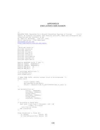
![129
if ((d<=350)&&(d>200)) return 20
if ((d<=350)&&(d>200)) return 20;
if ((d<=200)&&(d>55)) return 8;
if ((d<=55)&&(d>25)) return 4;
if ((d<=25)&&(d>0)) return 0;
}
float PLoss2(int n, float d){
if ((d<=490)&&(d>0))
return 0.0;
else
return 128.0;
}
/* for Distances greater than 300m n=n+1.3 */
/* Path Loss equation model with two values of n */
/* do =1 */
float PLoss(int n, float d){
/* it is only 20+ because we assume loss already from attenuators
antenna and physical media existing do=10 */
if (d<=20)
return 0;
if ((d>=20)&&(d<=450)){
return 10 + 10*n*log10(d); /* + 10*2.5*log10(10); att of local room */
}
if (d>450)
return 20+10*(n+1.3)*log10(d);
}
/* According to my lab this is the path loss */
/* */
float PLoss3(int n, float d){
float p;
p = PLoss(n, d);
if (p<=40)
return 0;
if (p>=95)
return 128;
return (55/55*p) - (55/35)*40;
}
/* Attenuation value to the Attenuator
50P-1230 has 1, 2,4, 8, 16, and 64dB per pin,
from the LSB to the MSB
50P-1230 has 1, 2,4, 8, 16, and 64dB per pin,
from the LSB to the MSB
*/
int Attenuator(float attenuation, int id){
int value=0;
if (attenuation<0)
value = 128;
else if (attenuation>127)
value = 255;
else value = 128 + (int) attenuation;
if (id!=0)
value = 128 + (255 - value) ; /* Attenuators 1 and 2 are inverted */
return value;
}
/* Structure for the baseStation info */
typedef struct {
float x, y;
char name[20];](https://image.slidesharecdn.com/hernandezefinal-100909142132-phpapp01/85/Adaptive-Networking-Protocol-for-Rapid-Mobility-142-320.jpg)
![130
int status; /* TRUE ON, FALSE OFF */
int power; /* 0=1mW, 1=5mW, 2=10mW, 3=20mW, 4=50mW, 5=100mW */
} baseStation;
typedef struct {
float initX;
float initY;
float currentX;
float currentY;
float speed;
float angle;
}mobileNode;
/* This area will read of the file to load the BS information */
baseStation** initializeBS(){
int i;
baseStation** bs;
bs = (baseStation**)malloc(MAX_BS_X*MAX_BS_Y*sizeof(baseStation*));
for (i=0;i<MAX_BS_X; i++)
bs[i] = (baseStation*) malloc(MAX_BS_Y*sizeof(baseStation));
bs[0]->x=500;
bs[0]->y=250;
bs[0]->status=0;
strcpy(bs[0]->name,"bs-1");
bs[0]->status=0;
strcpy(bs[0]->name,"bs-1");
bs[1]->x=1500;
bs[1]->y=250;
bs[1]->status=0;
strcpy(bs[1]->name,"bs-2");
bs[2]->x=2500;
bs[2]->y=250;
bs[2]->status=0;
strcpy(bs[2]->name,"bs-3");
bs[3]->x=3500;
bs[3]->y=250;
bs[3]->status=0;
strcpy(bs[3]->name,"bs-4");
bs[4]->x=4500;
bs[4]->y=250;
bs[4]->status=0;
strcpy(bs[4]->name,"bs-5");
bs[5]->x=5500;
bs[5]->y=250;
bs[5]->status=0;
strcpy(bs[5]->name,"bs-6");
bs[6]->x=6500;
bs[6]->y=250;
bs[6]->status=0;
strcpy(bs[6]->name,"bs-7");
bs[7]->x=7500;
bs[7]->y=250;
bs[7]->status=0;
strcpy(bs[7]->name,"bs-8");
bs[8]->x=8500;
bs[8]->y=250;
bs[8]->status=0;
strcpy(bs[8]->name,"bs-9");
return bs;
}
mobileNode* initializeMH(mobileNode* mh){
printf("%xn", mh);
mh->initX = 0.0;
mh->initY = 250.0;
mh->currentX = 0.0;
mh->currentY = 250.0;
mh->speed = 83.33333; /* in m/s */
mh->angle = 0.0; /* only 0 degress supported here */](https://image.slidesharecdn.com/hernandezefinal-100909142132-phpapp01/85/Adaptive-Networking-Protocol-for-Rapid-Mobility-143-320.jpg)
![131
return mh;
}
}
/* requires delta time in seconds */
void updatePosition(mobileNode* mh, float dtime) {
printf("MH at x=%f y=%f @%5.2fn", mh->currentX, mh->currentY, mh->speed);
mh->currentX= mh->speed * dtime + mh->currentX;
/* Angle not considered */
}
float distance(baseStation* bs, mobileNode* mh){
float d = sqrt(pow(mh->currentX-(bs->x),2) + pow(mh->currentY-(bs->y), 2));
/* printf("distance from %s %5.2f n", bs->name, d); */
return d;
}
/* emulation Code */
void runEmulation(baseStation** bs, mobileNode* mh, float granularity){
int i=0;
int j1=0;
int j2=1;
int j3=2;
double counter=0;
double elapsed=0;
float PathLoss1, PathLoss2, PathLoss3;
float dist1, dist2, dist3;
i=0;
printf("Initializing emulation @ T=0 n");
writePort(0); writePort(128);
writePort(1); writePort(128);
writePort(2); writePort(128);
printf("Running emulation.... in 10 seconds , start FA1, FA2, FA3 n");
for (i=0;i<=10;i++){
usleep(1000000);
printf("%d ...n",i+1);
}
printf("n Everybody must be associated to att0n");
printf("MH %x at x=%f y=%f speed=%fn", mh, mh->currentX, mh->currentY, mh->speed);
printf("Emulation granularity at %d secs ", (int) granularity/1000000);
printf("Emulation information :n Node 1 t Node 2 t Node 3 n");
printf("----------------------------------------------------------n");
while (mh->currentX<=8000) {
elapsed=rtc();
dist1 = distance(bs[j1], mh);
dist2 = distance(bs[j2], mh);
dist3 = distance(bs[j3], mh);
printf("n@@@@@@@@@@@@ ------->[ %8e ] --- ", elapsed);
/* I rather turn off the BS if it's out of range */
printf("n@@@@@@@@@@@@ ------->[ %8e ] --- ", elapsed);
/* I rather turn off the BS if it's out of range */
if ((dist1 >= 600) && (bs[j1]->status==0)){
printf("####### %s is going off n", bs[j1]->name);
StopAP(1);
bs[j1]->status = 1;
}
if ((dist1 < 600) && (bs[j1]->status==1)){
printf("####### %s is going ON n", bs[j1]->name);
StartAP(1);
bs[j1]->status = 0;
}
if ((dist1>=2000) && (dist1>dist2) && (dist1>dist3))
j1=j1+3;
/* Same with BS2 */
if ((dist2 >= 600) && (bs[j2]->status==0)){
printf("####### %s is going off n", bs[j2]->name);
StopAP(2);
bs[j2]->status = 1;
}
if ((dist2 < 600) && (bs[j2]->status==1)){](https://image.slidesharecdn.com/hernandezefinal-100909142132-phpapp01/85/Adaptive-Networking-Protocol-for-Rapid-Mobility-144-320.jpg)
![132
printf("####### %s is going ON n", bs[j2]->name);
StartAP(2);
bs[j2]->status = 0;
}
if ((dist2>=2000) && (dist2>dist1) && (dist2>dist3))
j2=j2+3;
/* Same with Bs3 */
if ((dist3 >= 600) && (bs[j3]->status==0)){
printf("###### %s is going off n", bs[j3]->name);
StopAP(3);
bs[j3]->status= 1;
}
if ((dist3 < 600) && (bs[j3]->status==1)){
printf("###### %s is going ON n", bs[j3]->name);
StartAP(3);
bs[j3]->status = 0;
}
if ((dist3>=2000) && (dist3>dist1) && (dist3>dist2) && (j1>j3))
j3=j3+3;
PathLoss1= PLoss2(3.5, distance(bs[j1], mh));
PathLoss2= PLoss2(3.5, distance(bs[j2], mh));
PathLoss3= PLoss2(3.5, distance(bs[j3], mh));
printf("Path Loss :");
printf(" %2.2f %2.2f %2.2f n", PathLoss1, PathLoss2, PathLoss3);
printf("Path Loss :");
printf(" %2.2f %2.2f %2.2f n", PathLoss1, PathLoss2, PathLoss3);
if (bs[j1]->status==0){
writePort(0);
writePort(Attenuator(PathLoss1, 0));
printf("Port 0 -> %d t", Attenuator(PathLoss1, 0));
}
if (bs[j2]->status==0){
writePort(1);
printf(" Port 1 -> %d t", Attenuator(PathLoss2, 1));
writePort(Attenuator(PathLoss2, 1));
}
if (bs[j3]->status==0){
printf("Port 2 -> %d t", Attenuator(PathLoss3, 2));
writePort(2);
writePort(Attenuator(PathLoss3, 2));
}
printf("n");
printf(" Bs->[%d] is %d bs->[%d] is %d, bs->[%d] is %d n", j1, bs[j1]-
>status, j2, bs[j2]->status, j3, bs[j3]->status );
printf("Distances: %2.2f %2.2f %2.2f n", distance(bs[j1], mh),
distance(bs[j2], mh), distance(bs[j3], mh));
updatePosition(mh, granularity/1000000); /* time in secs */
elapsed=rtc()-elapsed;
usleep(granularity-elapsed);
printf("Adjusting counter by %8f usec ", elapsed);
counter=0;
}
}
void StartAP(int Id){
pid_t pid;
if ((pid =fork())<0)
printf("Can't fork() -1 n");
else if (pid==0) {
/* printf("STOP APs %d.... n", Id); */
if (Id==1)
execl("/bin/bash","bash","-
c","/root/experiment_1/turnon_1>/dev/null","",NULL);
if (Id==2)
execl("/bin/bash","bash","-
c","/root/experiment_1/turnon_2>/dev/null","",NULL);
if (Id==3)](https://image.slidesharecdn.com/hernandezefinal-100909142132-phpapp01/85/Adaptive-Networking-Protocol-for-Rapid-Mobility-145-320.jpg)
![133
execl("/bin/bash","bash","-
c","/root/experiment_1/turnon_3>/dev/null","",NULL);
}
execl("/bin/bash","bash","-
c","/root/experiment_1/turnon_3>/dev/null","",NULL);
}
if (waitpid(pid, NULL, 0) < 0)
printf("wait error on AP %d n", Id);
}
void StopAP(int Id){
pid_t pid;
if ((pid =fork())<0)
printf("Can't fork() -1 n");
else if (pid==0) {
/* printf("STOP APs %d.... n", Id); */
if (Id==1)
execl("/bin/bash","bash","-
c","/root/experiment_1/turnoff_1>/dev/null","",NULL);
if (Id==2)
execl("/bin/bash","bash","-
c","/root/experiment_1/turnoff_2>/dev/null","",NULL);
if (Id==3)
execl("/bin/bash","bash","-
c","/root/experiment_1/turnoff_3>/dev/null","",NULL);
}
if (waitpid(pid, NULL, 0) < 0)
printf("wait error on AP %d n", Id);
}
int main(int argc, char **argv)
{
int i=0;
int j=0;
int k=0;
pid_t pid;
char IN[10];
baseStation** BS;
mobileNode* MH=(mobileNode*)malloc(sizeof(mobileNode));
/* Get access to the ports */
if (ioperm(BASEPORT, 3, 1))
{
perror("ioperm"); exit(1);
}
printf("[ RAMON ] - mobile network emulation environment n");
printf("Initializing BS.... n");
printf("[ RAMON ] - mobile network emulation environment n");
printf("Initializing BS.... n");
BS = initializeBS();
printf("Initializing MH.... n");
MH = initializeMH(MH);
printf("Starting APs .... if they were down, now are up n");
StartAP(1);
StartAP(2);
StartAP(3);
usleep(5000000);
printf("*-----> MH at speed < %2.2f >", MH->speed);
runEmulation(BS, MH, 1000000);
printf("----------------- going back to Att0 -------->n");
writePort(0); writePort(128);
writePort(1); writePort(128);
writePort(2); writePort(128);
StartAP(1);
StopAP(2);
StopAP(3);](https://image.slidesharecdn.com/hernandezefinal-100909142132-phpapp01/85/Adaptive-Networking-Protocol-for-Rapid-Mobility-146-320.jpg)
![APPENDIX C
MATLAB KALMAN FILTER FOR GHOST MN/FA
%Proof of the Kalman Filter
% Edwin Hernandez
% Basic kalman filter for the MIP implementation
% ---------------------------------------------------------------
t=0;
x_k=[0;
0;
20;
20];
w_k=[1;
2;
5;
5];
A=[1 0 t 0;
0 1 0 t;
0 0 1 0;
0 0 0 1];
H=[1 0 0 0;
0 1 0 0];
% Covariance matrix
P_k=eye(4);
% it's just an stimation;
z_k=[0;
0;];
v_k=[2;
1;];
% E{Wk Wk];
Q = [15 0 0 0;
0 15 0 0;
0 0 1 0;
0 0 0 1]
Q=Q*0.00001;
135](https://image.slidesharecdn.com/hernandezefinal-100909142132-phpapp01/85/Adaptive-Networking-Protocol-for-Rapid-Mobility-148-320.jpg)
![136
%E[vk vk'];
R = [100 0;
0 0.01];
R=R*0.0000001;
% Values of Time and speedx and speedy
% time x y
mvmnt = [0 0 0;
5 5 5;
10 14 24;
15 20 22;
20 45 60;
25 56 30;
30 70 70;
35 80 20;
50 60 140;
55 90 50;
60 90 4;
65 100 2;
70 120 10;
75 125 25
80 133 15;
85 142 20;
90 152 10;
95 10 22;];
[L,C]=size(mvmnt);
x=10;
y=40;
T=1;
t=0;
i=0;
while (t<95)
i=i+1;
t=t+T
j=0;
while (j<L-1)
j=j+1;
if ((t>=mvmnt(j,1))&(t<mvmnt(j+1,1)))
x=mvmnt(j,2)
y=mvmnt(j,3)
end
end
% x and y measured from the file.
x_measured(i, 1) = x;
x_measured(i, 2) = y;
z_k = [x y]';
% Predicted data
xp_k=A*x_k; %+ w_k;
PP_k=A*P_k*A' + Q;](https://image.slidesharecdn.com/hernandezefinal-100909142132-phpapp01/85/Adaptive-Networking-Protocol-for-Rapid-Mobility-149-320.jpg)
![LIST OF REFERENCES
[Aca94] Acampora A. and Naghshineh M. ”An architecture and methodology for
mobile-executed hand-off in cellular ATM networks,” IEEE Journal of
Selected Topics in Communications, Vol. 12, October 1994, pp.1365-1375.
[All97] Allman M., Caldwell A., and Ostermann S. “ONE: The Ohio Network
Emulator,” School of Electrical Engineering and Computer Science Ohio
University TR-19972, Columbus, Ohio, August 1997.
[Bahl00a] Bahl P., and Padmanabhan, V. “User Location and Tracking in an In-
Building Radio Network,” Proceedings of IEEE Infocom 2000, Piscataway,
NJ, March 2000, pp. 775-784.
[Bahl00b] Bahl P., Padmanabhan V., and Balachandran A., “A Software System for
Locating Mobile Users: Design, Evaluation, and Lessons”, Microsoft
Research Technical Report MSR-TR-2000-12, Redmond, Washington,
February 2000
[Bala95] Balakrishnan H., Seshan S., and Katz R., “Improving reliable transport and
handoff performance in cellular wireless networks,” ACM Wireless
Networks, Vol. 1, No. 4, December 1995.
[Bala96] Balakrishnan H., Padmanabhan V., Seshan S., and Katz R..”A comparison
of mechanisms for improving TCP performance over wireless links,”
Proceedings ACM SIGCOMM, Stanford, California, August 1996.
[Bha96] Bhagwat P., Perkins, C., and Tripathi, S., “Network Layer Mobility: An
architecture and Survey”, IEEE Personal Communications, Vol. 3. No. 3,
June 1996, pp. 54-64.
[Bing00] Bing B.. “High-speed wireless ATM and LANs”, Artech, Boston, MA,
2000.
[Broc98] Broch J., Johnson D. B., Maltz D. A., Hu J., and Jetcheva J.,”A
performance comparison of multi-hop wireless ad-hoc network routing
protocols”, Proceedings of MOBICOM 1998, Dallas, Texas, October. 1998,
pp. 85-97.
139](https://image.slidesharecdn.com/hernandezefinal-100909142132-phpapp01/85/Adaptive-Networking-Protocol-for-Rapid-Mobility-152-320.jpg)
![140
[Cace96a] Caceres R., and Iftode L.,” Improving the performance of reliable transport
protocols in mobile computing environments,” IEEE Journal of Selected
Areas in Communications, Vol. 13, No. 5, November 1996, pp. 850-857.
[Cace96b] Caceres R., and Padmanabhan V. "Fast and Scalable Handoffs for Wireless
Internetworks.", Proceedings of MOBICOM 1996, November 1996, pp. 56-
66.
[Camp00] Campbell A. T., Gomez J., Kim S., Turanyi Z., Wan C-Y. and Valko
A.,"Design, Implementation and Evaluation of Cellular IP", IEEE Personal
Communications, Special Issue on IP-based Mobile Telecommunications
Networks, Vol. 7, No. 4, August 2000, pp. 42-49.
[Camp01] Campbell A. T., and Gomez J.,"IP Micro-Mobility Protocols", ACM
SIGMOBILE Mobile Computer and Communication Review (MC2R),
Vol. 4, No. 4, October 2001, pp. 45-54.
[Camp02] Campbell A. T., Gomez, J., Kim, S., Turanyi, Z., Wan C-Y. and Valko
A.,"Comparison of IP Micro-Mobility Protocols," IEEE Wireless
Communications Magazine, Vol. 9, No. 1, February 2002.
[Cast98] Castelluccia C.. “A Hierarchical Mobile IPv6 proposal”, Technical Report
INRIA, France, November 1998.
[Chin02] Chinta M., Helal A., and Hernandez E.. “ILC-TCP: An Interlayer
Collaboration Protocol for TCP Performance Improvement in Mobile and
Wireless Environments,” Submitted to the Fifth ACM International
Workshop on Modeling, Analysis and Simulation of Wireless and Mobile
Systems , September 2002, Atlanta, Georgia.
[Cis01] CISCO Systems, Wireless Access Point,
http://www.cisco.com/univercd/cc/td/doc/pcat/ao350ap.htm, May 2002.
[Con00] J. Conrad, B.,Ullman C., Short S., Rama R., Schenken J., Harvey B.,
Hollis B., Glynn J., and Dengler P., “Introducing .NET,” WROX press,
Birmingham, UK, 2000.
[Dail99] Dailey D., Wall Z., Maclean S., and Cathey F., “An Algorithm and
Implementation to Predict the Arrival of Transit Vehicles,” IEEE ITSC'99,
Tokyo, Japan, 5-8, October 1999.
[Elma01] El Malki K., Calhoun P., Hiller T., Kempf J., McCann P., Singh A.,
Soliman H., and Thalanany, S., “Low Latency Handoff in Mobile IPv4,”
Internet draft submission, http://www.ietf.org/internet-drafts/draft-ietf-
mobileip-lowlatency-handoffs-v4-03.txt, November 2001.](https://image.slidesharecdn.com/hernandezefinal-100909142132-phpapp01/85/Adaptive-Networking-Protocol-for-Rapid-Mobility-153-320.jpg)
![141
[Erge02] Ergen M., Coleri S., Dundar B., Puri A., and Varaiya P., “Fast Handoff
with GPS routing for Mobile IP”, IPCN 2002, April 2002, Paris, France.
[Fall00] Fall K., and Varadhan K., “NS notes and documentation,” The VINT
project, Lawrence Berkeley Labs, February 2000.
http://www.isi.edu/nsnam/ns/
[Flad99] Fladenmuller A., and De Silva, R.,“The effect of Mobile IP handoffs on the
performance of TCP”, Mobile Networks and Applications, Vol. 4, No. 2,
May 1999, pp. 131-135.
[Fors99a] Forsberg, D., Malinen J.T., Malinen, J.K., Weckström, T., and Tiusanen,
M., “Distributing Mobility Agents Hierarchically under Frequent Location
Updates,” Sixth IEEE International Workshop on Mobile Multimedia
Communications (MOMUC'99), San Diego 1999.
[Fors99b] Forsberg, D, Malinen, J.T., Malinen, J.K., Weckström, T., and Tiusanen, M
“Dynamics – HUT Mobile IP Technical Document,” Internet draft
submission, October 1999.
[Garg00] Garg V., “IS-95 CDMA and CDMA2000: Cellular/PCS Systems
Implementation,” Prentice Hall, New York, NY, 2000.
[Gerl99] Gerla M., Chiang C., and Zhang L.,“Tree multicast strategies in mobile,
multihop wireless networks,” Mobile Networks and Applications, Vol.4,
No. 3, October 1999, pp. 193-207
[Glass00] Glass S., Hiller T., Jacobs A., and Perkins C,. “Mobile IP Authentication,
Authorization and Accounting – RFC 2977,” IETF - Network Working
Group, October 2000.
[Gun01] Gunnerson E., “A programmer’s Introduction to C#,” 2nd Ed, A! Press,
Berkeley, CA, 2001.
[Hern01] Hernandez E., and Helal A., "Examining Mobile IP Performance in
Rapidly Mobile Environments: The Case of a Commuter Train," IEEE
Conference in Local Computer Networks, November 2001, Tampa, FL.
[Hill02] Hillebrand F., “GSM & UMTS: The Creation of Global Mobile
Communications,” John Wiley and Son’s, New York, NJ, December 2001.
[Holl99] Holland G. and Vaidya N.,”Analysis of TCP performance over Mobile Ad-
Hoc networks,” Proceedings of Mobicom 1999, Seattle, WA, 1999, pp 219-
230.](https://image.slidesharecdn.com/hernandezefinal-100909142132-phpapp01/85/Adaptive-Networking-Protocol-for-Rapid-Mobility-154-320.jpg)
![142
[Ieee99a] IEEE-board, “Part11: Wireless LAN Medium Access Control (MAC) and
Physical Layer Specification (PHY),” Piscataway, New York, NJ, 1999.
[Ieee99b] IEEE-board, “Part11: Wireless LAN Medium Access Control (MAC) and
Physical Layer Specification (PHY), High-speed Physical Layer in the 5
GHz Band,” Piscataway, New York, 1999.
[Jaco88] Jacobson V., “Congestion avoidance and control,” Computer
Communications Review, Vol. 18, No. 4, August 1988, pp. 314 – 329.
[Jin99] Jing J., Helal A., and Elmagarmid A., “Client-Server Computing in Mobile
environments,” ACM Transactions on Database Systems, Vol. 31, No. 2,
June 1999.
[Ko98] Ko Y.B., and Vaidya N.,”Location-aided Routing (LAR) in Mobile Ad-hoc
Networks,” Proceedings of MOBICOM 1998, pp. 66-75, 1998
[Levi95] Levine D., Akyildiz I., and Naghshineh M., “Shadow cluster concept for
resource allocation and call admission in ATM-based wireless networks,”
Proceedings of the Annual International Conference on Mobile Computing
and Networking, Proceedings of MOBICOM 1995, New York, NY, pp.
142-150
[Lia99] Liang B., and Haass Z., “A predictive-distance based mobility management
for PCS networks,” IEEE INFOCOM’99, March 1999, pp 1-7.
[Liu98] Liu T., Bahl P., and Chlamtac I.,”Mobility Modeling, Location Tracking
and Trajectory Prediction in Wireless Networks,” IEEE Journal on Special
Areas in Communications, Vol. 16, No. 6, August 1998, pp. 922-936.
[Mon98] CMU Monarch Project “CMU wireless extension to ns”, Carnegie Mellon
University, August 1998. http://www.monarch.cs.cmu.edu/
[Nist01] National Institute of Standards, Network Emulator, http://www.nist.gov/,
May 2002.
[Nav97] Navas J., and Imielinski T., “GeoCast – Geographic Addressing and
Routing”, Proceedings MOBICOM 1997, September 1997, Hungary,
pp.66-76.
[Ori01] Orinoco Wireless, Wireless Card Specification,
ftp://ftp.orinocowireless.com/pub/docs/ORINOCO, May 2002.
[Pahl95] Pahlavan K., and Levesque A.,“Wireless Information Networks,” John
Wiley & Son’s, New York, 1995](https://image.slidesharecdn.com/hernandezefinal-100909142132-phpapp01/85/Adaptive-Networking-Protocol-for-Rapid-Mobility-155-320.jpg)
![143
[Paw02] Pawlikowski K., Jeong H, and Lee J., “On Credibility of Simulation
Studies of Telecommunication Networks,” IEEE Communications
Magazine, Vol. 40, No. 1, January 2002, pp.132-139.
[Perk95] Perkins C. E., and Luo K., “Using DHCP with computers that move,”
Wireless Networks, No.1, January, 1995, pp. 341-353.
[Perk96a] Perkins C. E., and Johnson D. B., “Mobility support in Ipv6,” Proceedings
of MOBICOM 1996, November 1996, New York, pp. 27-37.
[Perk96b] Perkins C. E., “IP mobility support,” RFC 2002, IBM, October 1996.
[Perk96c] Perkins C. E., “Mobile IP local registration with hierarchical foreign
agents,” Internet Draft, Internet Engineering Task Force, February 1996.
[Perk99] Perkins C. E. and Wang K.Y. “Optimized Smooth Handoffs in Mobile IP,”
Proceedings of the IEEE Symposium on Computers and Communications,
Red Sea, Egypt, July 1999.
[Perk01] Perkins C. E. and Johnson D., “Mobile IP Route Optimizations – internet –
draft,“ Internet draft submission, September 2001.
[Perk02] Perkins C. E., “IP support for mobility: RFC-3002,” IETF-RFC, January
2002.
[Ramj99] Ramjee R., La Porta T., Thuel S., Varadhan K., and Wang S., “HAWAII: A
Domain-based Approach for Supporting Mobility in Wide-area Wireless
Networks ,“ International Conference on Network Protocols ICNP'99,
October 199, Toronto, Canada.
[Ramj00] Ramjee R. , La Porta T., Thuel S., Varadhan K., and Salgarelli L., “IP
micro-mobility support using HAWAII ,” Internet draft submission, IETF,
Jul 2000.
[Rapp02] Rappaport T., “Wireless Communications: Principles and Applications,”
Prentice Hall, New Jersey, 2002.
[Reza95] Rezaiifar R., Makowski A., and Kumar S.,“Stochastic Control of Handoffs
in Cellular Networks,” IEEE Journal of Selected Areas in Communication,
Vol. 13, No. 7, September 1995, pp.1348-1362.
[Shah02] Shah S., Hernandez E., and Helal A., "CAD-HOC: A CAD Like Tool for
Generating Mobility Benchmarks in Ad-Hoc Networks," Proceedings of
the second IEEE/IPSJ Symposium on Applications and the Internet
(SAINT'02), February 2002, Nara, Japan.](https://image.slidesharecdn.com/hernandezefinal-100909142132-phpapp01/85/Adaptive-Networking-Protocol-for-Rapid-Mobility-156-320.jpg)
![144
[Snoe01] Snoeren A., Balakrishnan H., and Frans M., “Reconsidering Internet
Mobility,” Proceedings of the 8th Workshop on Hot Topics in Operating
Systems, Germany, May 2001.
[Sta00] Stallings C., “Computer Communication Networks,” McGraw Hill, New
York, 2001.
[Solo98] Solomon J. “Mobile IP,” Prentice Hall, New Jersey, 1998.
[Su00] Su W., Lee S., and Gerla N., ”Mobility Prediction in Wireless Networks,”
Proceedings of IEEE MILCOM 2000, Los Angeles, CA, Oct. 2000.
[Terz99] Terzis A., Srivastava M., and Zhang L., “A Simple QoS Signaling Protocol
for Mobile Hosts in the Integrated Services Internet,” Proceedings of IEEE
INFOCOM99, March 1999.
[Valk98] Valko A. G., Campbell A., and Gomez J., "Cellular IP," Internet Draft,
draft-valko-cellularip-00.txt, November 1998.
[Valk99] Valko A. G., "Cellular IP - A New Approach to Internet Host Mobility,"
ACM Computer Communication Review, Vol. 29, No. 1, January 1999, pp.
50-65.
[Wan98] Wan Y., Chen W., and Ho J. “Performance analysis of Mobile IP extended
with routing agents,” Proceedings of the 2nd European IASTED
International Conference on Parallel and Distributed Systems, July 1998
[Widm00] Widmer J. “Network simulations for a mobile network architecture for
vehicles,” TR-00-09 International Computer Science Institute, Berkeley,
CA, May 2000.
[Welc02] Welch G., and Bishop G.. “An Introduction to the Kalman Filter,”
University of North Carolina TR 95-041, UNC, Chapell Hill, North
Carolina, 2002.
[Wu01] Wu, J, Chen C., Huang N., and Ma G., “Intelligent handoff for Mobile
Wireless Internet,” Mobile Networks and Applications, Vol. 6, No. 2,
March 2001, pp. 67-79.
[Yeom01] Yeom I., and Reddy A. “ENDE: An End-to-End Network Delay
Emulator,” Multimedia Tools and Application, No.14, April 2001, pp. 269-
296.](https://image.slidesharecdn.com/hernandezefinal-100909142132-phpapp01/85/Adaptive-Networking-Protocol-for-Rapid-Mobility-157-320.jpg)

This document summarizes Edwin Hernandez-Mondragon's dissertation which proposes improvements to networking protocols for rapidly moving environments. The dissertation presents two contributions: 1) The Rapid Mobility Network Emulator (RAMON) which combines emulation and simulation to facilitate analysis of wireless protocol performance under high speed and mobility. RAMON allows controlling factors like attenuation and latency. 2) A predictive extension of Mobile IP using Kalman filtering to forecast speed and trajectory, enabling preemptive actions and improving performance at speeds up to 80m/s. Experiments show the predictive Mobile IP improves performance by at least 30% over the standard protocol.


![Network design for_ip_convergence[1]](https://cdn.slidesharecdn.com/ss_thumbnails/networkdesignforipconvergence1-100822173922-phpapp01-thumbnail.jpg?width=640&height=640&fit=bounds)