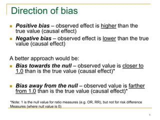
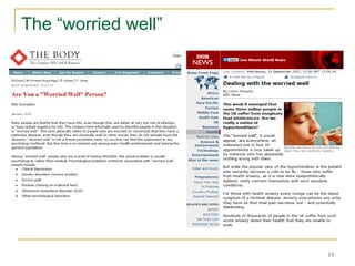
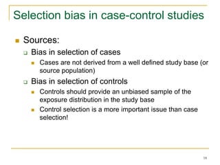
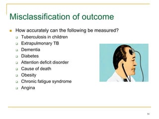
This document discusses various types of bias that can occur in epidemiological studies, including selection bias and information bias. Selection bias occurs when the study population is not representative of the target population, such as when there are differential participation rates related to exposure or disease status. Information bias, also called misclassification bias, arises from errors in measuring or recording exposure, disease status, or other variables. There is often no perfect way to measure exposures, and tools to assess past exposures like diet are especially imprecise. The direction and magnitude of bias introduced can impact study results and conclusions.

1. 1
Bias in Epidemiological
Studies
Madhukar Pai, MD, PhD
Associate Professor, Epidemiology
Associate Director, McGill International TB Centre
McGill University, Montreal, Canada
Email: madhukar.pai@mcgill.ca

2. 2
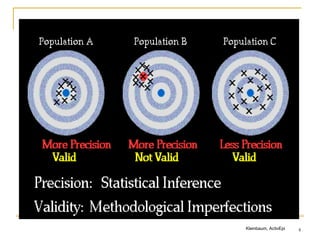
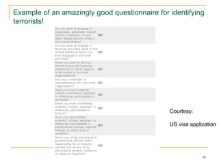
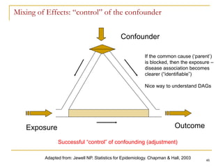
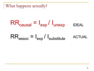
Adapted from: Maclure, M, Schneeweis S. Epidemiology 2001;12:114-122.
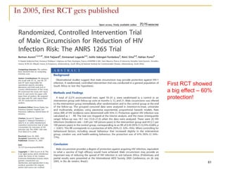
Causal Effect
Random Error
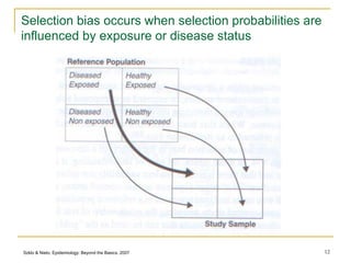
Selection bias
Information bias
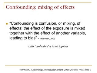
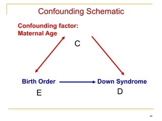
Confounding
Bias in analysis & inference
Reporting & publication bias
Bias in knowledge use
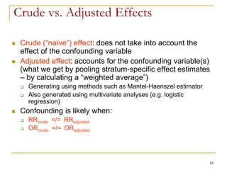
The long road to causal inference
(the “big picture”)
RRcausal
“truth”
[counterfactual]
RRassociation
the long road to causal inference…
BIAS

3. 3
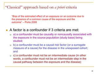
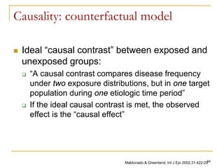
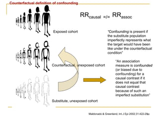
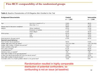
Error
Systematic error
Random error
Information
bias
Selection bias
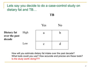
Errors in epidemiological inference
Confounding
BIAS
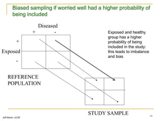
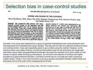
“Bias is any process at any stage of inference which tends to produce results or
conclusions that differ systematically from the truth” – Sackett (1979)
“Bias is systematic deviation of results or inferences from truth.” [Porta, 2008]
PRECISION:
defined as relative
lack of random
error
VALIDITY: defined as
relative absence of bias
or systematic error

4. 4
Kleinbaum, ActivEpi

5. 5
Direction of bias
 Positive bias – observed effect is higher than the
true value (causal effect)
 Negative bias – observed effect is lower than the true
value (causal effect)
A better approach would be:
 Bias towards the null – observed value is closer to
1.0 than is the true value (causal effect)*
 Bias away from the null – observed value is farther
from 1.0 than is the true value (causal effect)*
*Note: 1 is the null value for ratio measures (e.g. OR, RR), but not for risk difference
Measures (where null value is 0)

6. 6
Selection Bias in
Epidemiological Studies

7. 7
“….nearly half had to support the daily hospitalization cost, that cannot be
afforded by all patients and has lead to an obvious bias. We have also gathered
data from patients moving from the National Tuberculosis Center to the French
Military Hospital and this could lead to an overestimation of the MDR rate.”

8. 8
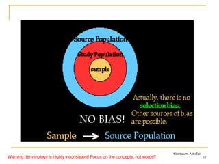
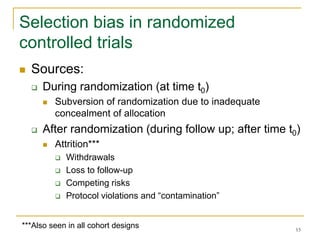
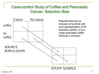
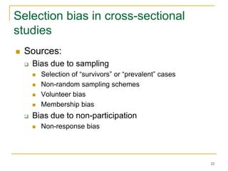
Now lets define selection bias
 “Distortions that result from procedures used to select
subjects and from factors that influence participation in
the study.”
 Porta M. A dictionary of epidemiology. Oxford, 2008.
 “Error introduced when the study population does not
represent the target population”
 Delgado-Rodriguez et al. J Epidemiol Comm Health 2004
 Defining feature:
 Selection bias occurs at:
 the stage of recruitment of participants
 and/or during the process of retaining them in the study
 Difficult to correct in the analysis, although one can do sensitivity
analyses
Who gets picked for a study, who refuses, who agrees, who stays in a
study, and whether these issues end up producing a “skewed” sample that
differs from the target [i.e. biased study base].

9. 9
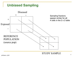
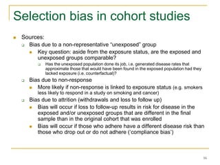
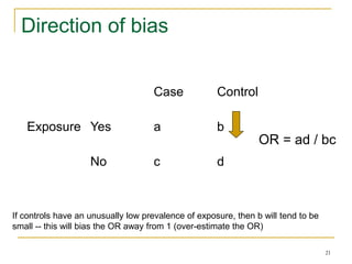
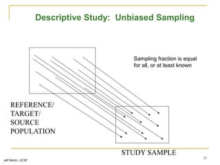
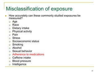
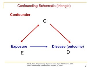
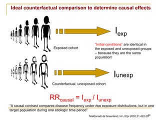
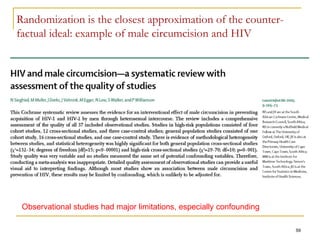
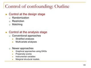
Hierarchy of populations
Target (external) population
[to which results may be generalized]
Source
population
(source base)**
Eligible
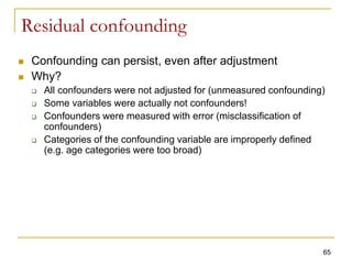
population
(intended sample;
possible to get
all)
Actual study
population
(study sample
successfully
enrolled)
**The source population may be defined directly, as a matter of defining its membership criteria; or the
definition may be indirect, as the catchment population of a defined way of identifying cases of the illness.
The catchment population is, at any given time, the totality of those in the ‘were-would’ state of: were the
illness now to occur, it would be ‘caught’ by that case identification scheme [Source: Miettinen OS, 2007]
Study base, a
series of person-
moments within the
source base (it is
the referent of the
study result)
Warning: terminology is highly inconsistent! Focus on the concepts, not words!!

10. 10
Warning: terminology is highly inconsistent! Focus on the concepts, not words!!
Kleinbaum, ActivEpi

11. 11
Diseased
Exposed
+ -
+
-
REFERENCE
POPULATION
(source pop)
STUDY SAMPLE
Unbiased Sampling
Jeff Martin, UCSF
Sampling fractions
appear similar for all
4 cells in the 2 x 2 table

12. 12
Selection bias occurs when selection probabilities are
influenced by exposure or disease status
Szklo & Nieto. Epidemiology: Beyond the Basics. 2007

13. The “worried well”
13

14. 14
Diseased
Exposed
+ -
+
-
REFERENCE
POPULATION
STUDY SAMPLE
Biased sampling if worried well had a higher probability of
being included
Jeff Martin, UCSF
Exposed and healthy
group has a higher
probability of being
included in the study:
this leads to imbalance
and bias

15. 15
Selection bias in randomized
controlled trials
 Sources:
 During randomization (at time t0)
 Subversion of randomization due to inadequate
concealment of allocation
 After randomization (during follow up; after time t0)
 Attrition***
 Withdrawals
 Loss to follow-up
 Competing risks
 Protocol violations and “contamination”
***Also seen in all cohort designs

16. 16
Selection bias in cohort studies
 Sources:
 Bias due to a non-representative “unexposed” group
 Key question: aside from the exposure status, are the exposed and
unexposed groups comparable?
 Has the unexposed population done its job, i.e. generated disease rates that
approximate those that would have been found in the exposed population had they
lacked exposure (i.e. counterfactual)?
 Bias due to non-response
 More likely if non-response is linked to exposure status (e.g. smokers
less likely to respond in a study on smoking and cancer)
 Bias due to attrition (withdrawals and loss to follow up)
 Bias will occur if loss to follow-up results in risk for disease in the
exposed and/or unexposed groups that are different in the final
sample than in the original cohort that was enrolled
 Bias will occur if those who adhere have a different disease risk than
those who drop out or do not adhere (‘compliance bias’)

17. 17
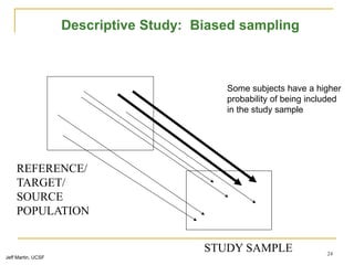
Healthy User and Healthy Continuer Bias:
HRT and CHD
 HRT was shown to reduce coronary heart disease (CHD) in women in
several observational studies
 Subsequently, RCTs showed that HRT might actually increase the risk of
heart disease in women
 What can possibly explain the discrepancy between observational and
interventional studies?
 Women on HRT in observational studies were more health conscious, thinner,
and more physically active, and they had a higher socioeconomic status and
better access to health care than women who are not on HRT
 Self-selection of women into the HRT user group could have generated
uncontrollable confounding and lead to "healthy-user bias" in observational
studies.
 Also, individuals who adhere to medication have been found to be healthier than
those who do not, which could produce a "compliance bias” [healthy user bias]
Michels et al. Circulation. 2003;107:1830

18. 18
Selection bias in case-control studies
 Sources:
 Bias in selection of cases
 Cases are not derived from a well defined study base (or
source population)
 Bias in selection of controls
 Controls should provide an unbiased sample of the
exposure distribution in the study base
 Control selection is a more important issue than case
selection!

19. 19
Selection bias in case-control studies
MacMahon et al. N Engl J Med. 1981 Mar 12;304(11):630-3
Controls in this study were selected from a group of patients hospitalized by the same physicians who
had diagnosed and hospitalized the cases' disease. The idea was to make the selection process of cases
and controls similar. It was also logistically easier to get controls using this method. However, as the
exposure factor was coffee drinking, it turned out that patients seen by the physicians who diagnosed
pancreatic cancer often had gastrointestinal disorders and were thus advised not to drink coffee (or had
chosen to reduce coffee drinking by themselves). So, this led to the selection of controls with higher
prevalence of gastrointestinal disorders, and these controls had an unusually low odds of exposure
(coffee intake). These in turn may have led to a spurious positive association between coffee intake and
pancreatic cancer that could not be subsequently confirmed.

20. 20
Cancer No cancer
coffee
no
coffee
SOURCE
POPULATION
STUDY SAMPLE
Case-control Study of Coffee and Pancreatic
Cancer: Selection Bias
Jeff Martin, UCSF
Potential bias due to
inclusion of controls with
over-representation of GI
disorders (which, in turn,
under-estimated coffee
drinking in controls)

21. 21
Direction of bias
Case Control
Exposure Yes a b
No c d
If controls have an unusually low prevalence of exposure, then b will tend to be
small -- this will bias the OR away from 1 (over-estimate the OR)
OR = ad / bc

22. 22
Selection bias in cross-sectional
studies
 Sources:
 Bias due to sampling
 Selection of “survivors” or “prevalent” cases
 Non-random sampling schemes
 Volunteer bias
 Membership bias
 Bias due to non-participation
 Non-response bias

23. 23
REFERENCE/
TARGET/
SOURCE
POPULATION
STUDY SAMPLE
Descriptive Study: Unbiased Sampling
Jeff Martin, UCSF
Sampling fraction is equal
for all, or at least known

24. 24
REFERENCE/
TARGET/
SOURCE
POPULATION
STUDY SAMPLE
Descriptive Study: Biased sampling
Jeff Martin, UCSF
Some subjects have a higher
probability of being included
in the study sample

25. 25
Information Bias in
Epidemiological Studies
“Bias in an estimate arising from measurement errors”
Porta M. A dictionary of epidemiology. Oxford, 2008.

26. 26
Example of an amazingly good questionnaire for identifying
terrorists!
Courtesy:
US visa application

27. 27
Lets say you decide to do a case-control study on
dietary fat and TB…
TB
Yes No
Dietary fat
over the past
decade
High a b
Low c d
How will you estimate dietary fat intake over the past decade?
What tools could you use? How accurate and precise are these tools?
Is the study worth doing???

28. 28
Misclassification of exposure
 How accurately can these commonly studied exposures be
measured?
 Age
 Race
 Dietary intake
 Physical activity
 Pain
 Stress
 Socioeconomic status
 Smoking
 Alcohol
 Sexual behavior
 Adherence to medications
 Caffeine intake
 Blood pressure
 Intelligence

29. 29
How to measure adherence?
 Is there a gold standard?
 No gold standard method
 What are the available methods?
 Provider’s assessment of adherence
 Self reported adherence by patient
 Standardized, patient-administered questionnaires
 Pill counts (e.g. remaining dosage units)
 Pharmacy database (prescription refills, etc)
 MEMS (medication event monitoring system)
 Biochemical measurements (e.g. biomarkers in urine)
 Direct observation of medication ingestion (e.g. DOT)
 Which approach is most prone to misclassification?
 Provider’s assessment of adherence
 Which approach is least prone to misclassification?
 DOT, MEMS
 What may be the optimal strategy, considering cost and feasibility?
 Overall, no single measurement strategy is optimal
 multi-method approach that combines self-reporting with some objective
measure is the current state-of-the-art in measurement of adherence
Source: WHO, 2003

30. 30
Misclassification of outcome
 How accurately can the following be measured?
 Tuberculosis in children
 Extrapulmonary TB
 Dementia
 Diabetes
 Attention deficit disorder
 Cause of death
 Obesity
 Chronic fatigue syndrome
 Angina

31. 31
So, its important to note that in all epi
studies:
 Exposure will be measured with some
sensitivity and some specificity
 Disease will be measured with some
sensitivity and some specificity
 Confounders (covariates) will be measured
with some sensitivity and some specificity
 If each is measured with error, then imagine
how they can all add up!

32. 32
Information bias in randomized
controlled trials
 Sources:
 Lack of blinding can cause detection bias (knowledge of
intervention can influence assessment or reporting of
outcomes)
 Subjects (“participant expectation bias”)
 Investigators
 Outcome assessors (“observer bias”)
 Data analysts
 Key issue: how “hard” is the outcome variable?
 Strong versus “soft” outcomes
 Blinding is very important for soft outcomes

33. 33
Information bias in cohort studies
 Sources:
 Misclassification of exposure at baseline (not likely to be
influenced by outcome status, because outcome has not
occurred)
 Changes in exposure status over time (time-dependent
covariates; dynamic exposures)
 Ascertainment of outcomes during follow-up (which can be
influenced by knowledge of exposure status: “detection bias” or
“outcome identification bias” or “diagnostic suspicion bias”)
 Clinical example: pathologist more likely to use the term
“tuberculous granuloma” when evaluating a specimen if the
pathologist knows the patient is a smoker and is a household
contact of a TB case

34. 34
Information bias in case-control
studies
 Sources:
 Poor recall of past exposures (poor memory; can happen
with both cases and controls; so, non-differential)
 Differential recall between cases and controls (“recall bias”
or “exposure identification bias” or “exposure suspicion
bias”)
 Cases have a different recall than controls
 Differential exposure ascertainment (influenced by
knowledge of case status)
 Interviewer/observer bias (cases are probed differently than
controls)

35. Non-differential misclassification bias
 Non-differential misclassification of disease:
 Sensitivity and Specificity for misclassifying
disease do not differ by exposure
 Non-differential misclassification of exposure:
 Sensitivity and Specificity for misclassifying
exposure do not differ by disease
 Non-differential misclassification of BOTH
disease and exposure leads to:
 Bias towards the null
35
Kleinbaum, ActivEpi

36. Differential misclassification bias
 With differential misclassification, either:
 Sensitivity and specificity for misclassifying
disease differs by exposure status
Or
 Sensitivity and specificity for misclassifying
exposure differs by disease status
 Differential misclassification of either disease or
exposure can lead to bias either towards the null
or away from the null
36
Kleinbaum, ActivEpi

37. 37
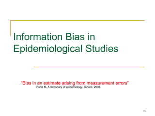
Reducing information bias
 Use the best possible tool to measure exposure and outcomes
 Use objective (“hard”) measures as much as possible
 Use blinding as often as possible, especially for soft outcomes
 Train interviewers and perform standardization (pilot) exercises
 Use the same procedures for collecting exposure information from
cases and controls [case-control study]
 Use the same procedures to diagnose disease outcomes in
exposed and unexposed [cohort study and RCTs]
 Collect data on sensitivity and specificity of the measurement tool
(i.e. validation sub-studies)
 Correct for misclassification by “adjusting” for imperfect sensitivity
and specificity of the tool
 Perform sensitivity analysis: range of plausible estimates given
misclassification

38. 38
Confounding in health
research

39. 39
Confounding:
4 ways to understand it!
1. “Mixing of effects”
2. “Classical” approach based on a priori
criteria
3. Collapsibility and data-based criteria
4. “Counterfactual” and non-comparability
approaches

40. 40
Confounding: mixing of effects
 “Confounding is confusion, or mixing, of
effects; the effect of the exposure is mixed
together with the effect of another variable,
leading to bias” - Rothman, 2002
Rothman KJ. Epidemiology. An introduction. Oxford: Oxford University Press, 2002
Latin: “confundere” is to mix together

41. 41
Example
Association between birth order and Down syndrome
Source: Rothman 2002
Data from Stark and Mantel (1966)

42. 42
Source: Rothman 2002
Association between maternal age and Down syndrome
Data from Stark and Mantel (1966)

43. 43
Source: Rothman 2002
Association between maternal age and Down syndrome, stratified by
birth order
Data from Stark and Mantel (1966)

44. 44
Mixing of Effects: the water pipes analogy
Adapted from Jewell NP. Statistics for Epidemiology. Chapman & Hall, 2003
Exposure Outcome
Confounder
Mixing of effects – cannot separate the effect of exposure from that of confounder
Exposure and disease
share a common cause (‘parent’)

45. 45
Mixing of Effects: “control” of the confounder
Adapted from: Jewell NP. Statistics for Epidemiology. Chapman & Hall, 2003
Exposure Outcome
Confounder
Successful “control” of confounding (adjustment)
If the common cause (‘parent’)
is blocked, then the exposure –
disease association becomes
clearer (“identifiable”)
Nice way to understand DAGs

46. 46
“Classical” approach based on a priori criteria
 A factor is a confounder if 3 criteria are met:
 a) a confounder must be causally or noncausally associated with
the exposure in the source population (study base) being
studied;
 b) a confounder must be a causal risk factor (or a surrogate
measure of a cause) for the disease in the unexposed cohort;
and
 c) a confounder must not be an intermediate cause (in other
words, a confounder must not be an intermediate step in the
causal pathway between the exposure and the disease)
“Bias of the estimated effect of an exposure on an outcome due to
the presence of a common cause of the exposure and the
outcome” – Porta 2008

47. 47
Exposure Disease (outcome)
Confounder
Confounding Schematic (triangle)
E D
C
Szklo M, Nieto JF. Epidemiology: Beyond the basics. Aspen Publishers, Inc., 2000.
Gordis L. Epidemiology. Philadelphia: WB Saunders, 4th Edition.

48. 48
Exposure
Confounder
General idea: a confounder is a ‘parent’ or
‘ancestor’ of the exposure and outcome, but
should not be a ‘child’ or ‘descendant’ of the
exposure or outcome
E D
C
Disease

49. 49
Birth Order Down Syndrome
Confounding factor:
Maternal Age
Confounding Schematic
E D
C

50. 50
Nutritional status Tuberculosis
Confounding factor:
SES
Are confounding criteria met?
Association between nutritional status and TB

51. 51
NRAMP1 gene Tuberculosis
Confounding factor:
Age
Are confounding criteria met?
x
Should we adjust for age, when evaluating the association
between a genetic factor and risk of TB?
No!

52. 52
Collapsibility and data-based approaches
 According to this definition, a factor is a confounding
variable if
 a) the effect measure is homogeneous across the strata
defined by the confounder and
 b) the crude and common stratum-specific (adjusted) effect
measures are unequal (this is called “lack of collapsibility”)
 Usually evaluated using 2x2 tables, and simple
stratified analyses to compare crude effects with
adjusted effects
“Collapsibility is equality of stratum-specific measures of effect with the crude
(collapsed), unstratified measure” Porta, 2008, Dictionary

53. 53
Crude vs. Adjusted Effects
 Crude (“naïve”) effect: does not take into account the
effect of the confounding variable
 Adjusted effect: accounts for the confounding variable(s)
(what we get by pooling stratum-specific effect estimates
– by calculating a “weighted average”)
 Generating using methods such as Mantel-Haenszel estimator
 Also generated using multivariate analyses (e.g. logistic
regression)
 Confounding is likely when:
 RRcrude =/= RRadjusted
 ORcrude =/= ORadjusted

54. 54
Causality: counterfactual model
 Ideal “causal contrast” between exposed and
unexposed groups:
 “A causal contrast compares disease frequency
under two exposure distributions, but in one target
population during one etiologic time period”
 If the ideal causal contrast is met, the observed
effect is the “causal effect”
Maldonado & Greenland, Int J Epi 2002;31:422-29

55. 55
Iexp
Iunexp
Counterfactual, unexposed cohort
Exposed cohort
Ideal counterfactual comparison to determine causal effects
RRcausal = Iexp / Iunexp
“A causal contrast compares disease frequency under two exposure distributions, but in one
target population during one etiologic time period”
Maldonado & Greenland, Int J Epi 2002;31:422-29
“Initial conditions” are identical in
the exposed and unexposed groups
– because they are the same
population!

56. 56
Iexp
Iunexp
Counterfactual, unexposed cohort
Exposed cohort
Substitute, unexposed cohort
Isubstitute
What happens actually?
counterfactual state
is not observed
A substitute will usually be a population other than the target population
during the etiologic time period - INITIAL CONDITIONS MAY BE
DIFFERENT

57. 57
What happens actually?
RRassoc = Iexp / Isubstitute
RRcausal = Iexp / Iunexp IDEAL
ACTUAL

58. 58
Counterfactual, unexposed cohort
Exposed cohort
Substitute, unexposed cohort
“Confounding is present if
the substitute population
imperfectly represents what
the target would have been
like under the counterfactual
condition”
“An association
measure is confounded
(or biased due to
confounding) for a
causal contrast if it
does not equal that
causal contrast
because of such an
imperfect substitution”
Maldonado & Greenland, Int J Epi 2002;31:422-29
Counterfactual definition of confounding
RRcausal =/= RRassoc

59. 59
Randomization is the closest approximation of the counter-
factual ideal: example of male circumcision and HIV
Observational studies had major limitations, especially confounding

60. 60
Confounders considered in the Cochrane review
Siegfried N et al. Lancet Infect Dis 2005

61. 61
In 2005, first RCT gets published
First RCT showed
a big effect – 60%
protection!

62. 62
Randomization resulted in highly comparable
distribution of potential confounders; so
confounding is not an issue (at baseline)
First RCT: comparability of the randomized groups

63. Control of confounding: Outline
 Control at the design stage
 Randomization
 Restriction
 Matching
 Control at the analysis stage
 Conventional approaches
 Stratified analyses
 Multivariate analyses
 Newer approaches
 Graphical approaches using DAGs
 Propensity scores
 Instrumental variables
 Marginal structural models
63

64. Control of confounding: at the analysis stage
 Unlike selection and information bias, confounding is one
type of bias that can be, to a large extent, adjusted in the
analysis
 Options at the analysis stage:
 Stratification
 Multivariate methods
 To control for confounding in the analyses, one must
measure the confounders in the study!
 Investigators usually do this by collecting data on all known,
previously identified confounders
 A sound knowledge of disease biology will help decide what to
measure
 Drawing a DAG before a study is done will help decide on what
minimum set of covariates need to be measured
64

65. Residual confounding
 Confounding can persist, even after adjustment
 Why?
 All confounders were not adjusted for (unmeasured confounding)
 Some variables were actually not confounders!
 Confounders were measured with error (misclassification of
confounders)
 Categories of the confounding variable are improperly defined
(e.g. age categories were too broad)
65

66. Residual confounding: a case study
66

67. Residual confounding: a case study
AJRCCM 2004 67

68. 68

69. Case studies on bias:
69
Real life case studies of how things went wrong and what we can learn from them!
Available at: www.teachepi.org

70. 70
Bias analysis and correction
(sensitivity analysis)
Applying Quantitative Bias Analysis to Epidemiologic Data
Springer, 2009
Lash, Timothy L., Fox, Matthew P., Fink, Aliza K.