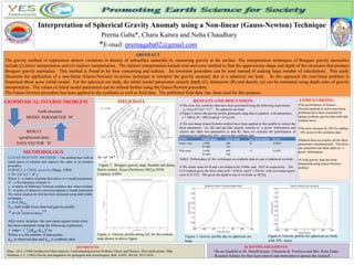
This document summarizes a study that uses a non-linear Gauss-Newton technique to interpret spherical gravity anomalies. It generates synthetic gravity data for a spherical ore body and applies the Gauss-Newton method to extract parameters like depth and dimension. When applied to noise-free data, the method accurately resolves the parameters in 22 iterations with low error. Adding 10% noise increases the error by 20% but parameters are still estimated reasonably well. The method is also applied to interpret a published field gravity dataset from Texas.

1. Interpretation of Spherical Gravity Anomaly using a Non-linear (Gauss-Newton) Technique
Prerna Gaba*, Charu Kamra and Neha Chaudhary
*E-mail: prernagaba02@gmail.com
Earth structure
MODEL PARAMETER ‘M’
RESULT
(geophysical data)
DATA VECTOR ‘D’
GEOPHYSICAL INVERSE PROBLEM
METHODOLOGY
GAUSS-NEWTON METHOD : The method start with an
initial guess of solution and improve the same in an iterative
procedure.
FORMULA USED: given by (Meju, 1994)
 X= (AT A ) -1 AT y
Where A : is matrix of partial derivatives w.r.t model parameters,
AT : is the transpose of matrix A
y : is matrix of difference between synthetic and observed data;
X : is matrix of unknown correction applied to model parameters
The initial solution for this has been estimated using half-width
technique.
 Z=1.3X1/2,
X1/2:half-width from observed gravity profile
 R=(3Z
2
G(MAX)/4Πγρ)
1/3
After every iteration the root mean square (rms) error
has been estimated using the following expression:
 rms= √ ∑(dobs-dsyn)2 /n
Where n is the number of data points
dobs is observed data and dsyn is synthetic data
FIELD DATA CONCLUSIONS:
•The performance of (Gauss -
Newton,method) to solve non-linear
problems have been examined by
taking synthetic gravity data with and
without noise.
•The error increase by 20% by adding
10% noise to the synthetic data
•Method does not resolve all the three
parameters simultaneously. Therefore,
one parameter has been taken as ‘a
priori’ information.
•A field gravity data has been
interpreted using Gauss-Newton
method
REFERENCES:
Meju , M.A. (1994) Geophysical Data Analysis: Understanding Inverse Problem Theory and Practice, SEG publications, 296p
Nettleton, L.L. (1962) Gravity and magnetics for geologists and seismologists: Bull. AAPG, 46(10), 1815-1838.
RESULTS AND DISCUSSION:
The noise free synthetic data have been generated using the following expressions:
gs=4πρzR3/3(x2+z2)3/2 for spherical ore body
Figure 3 shows the gravity profile generated using above equation with parameters
z = 500 m, R = 200 m and ρ = 0.4 g/cm3
The non-linear Gauss-Newton method have been applied to this profile to extract the
three parameters (z), (R) and (ρ).Take density contrast as ‘a priori’ information and
resolve the other two parameters (z and R). Next we examine the performance of
techniques by adding the 10% error to the synthetic data
Table1. Performance of the techniques on synthetic data in case of spherical ore body.
The initial value for R and z are found to be 3140m. and 5632 m respectively. The
G-N method gives the final value as R = 4581m. and Z = 8414m. with root mean square
error of 0.5353. This gives the depth to top of ore body as 3833m.
ABSTRACT
The gravity method of exploration detects variations in density of subsurface materials by measuring gravity at the surface. The interpretation techniques of Bouguer gravity anomalies
include (i) direct interpretation and (ii) indirect interpretation. The indirect interpretation include trial and error method to find the approximate shape and depth of the structures that produce
Bouguer gravity anomalies. This method is found to be time consuming and tedious. An inversion procedure can be used instead of making large number of calculations. This study
illustrates the application of a non-linear (Gauss-Newton) inversion technique to interpret the gravity anomaly due to a spherical ore body. In this approach the non-linear problem is
linearised about some initial model. For the spherical ore body, the initial model parameters namely depth (Z), dimension (R) and density () can be estimated using depth rules of gravity
interpretation. The values of initial model parameters can be refined further using the Gauss-Newton procedure.
The Gauss-Newton procedure has been applied to the synthetic as well as field data. The published field data has been used for this purpose.
Figure 1: Bouguer gravity map, Humble salt dome,
Harris county, Texas (Nettleton,1962,p.1839).
Courtesy AAPG
Figure 2: Gravity profile along AA’ for the contour
map shown in above figure
Figure 4: Gravity profile for spherical ore body
with 10% noise
Figure 3: Gravity profile due to spherical ore
body
ACKNOWLEDGEMENTS
We are thankful to Dr. Dinesh Kumar Chairman & Professor and Mrs. Renu Yadav
Research Scholar for their keen interest and motivation to pursue this research.
DATA Initial guess Final value No. of iterations Error
Noise –free z=800
R=400
500
216
22 0.0036
With noise z=800
R=400
669
246
13 0.0302