science, beer's, Beer's law

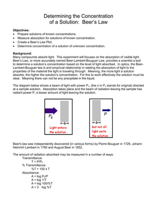
1. Determining the Concentration
of a Solution: Beer’s Law
Objectives:
· Prepare solutions of known concentrations.
· Measure absorption for solutions of known concentration.
· Create a Beer’s Law Plot.
· Determine concentration of a solution of unknown concentration.
Background:
Many compounds absorb light. This experiment will focuses on the absorption of visible light.
Beer’s Law, or more accurately named Beer-Lambert-Bouguer Law, provides a scientist a tool
to determine a solution’s concentration based on the level of light absorbed. In optics, the Beer-
Lambert-Bouguer law is and empirical relationship in relating the absorption of light to the
properties of the material the light is traveling through. Meaning, the more light a solution
absorbs, the higher the solution’s concentration. For this to work effectively the solution must be
clear. Meaning there can not be any precipitate in the liquid.
The diagram below shows a beam of light with power Po, (the o in Po stands for original) directed
at a sample solution. Absorption takes place and the beam of radiation leaving the sample has
radiant power P, a lesser amount of light leaving the solution.
Beer's law was independently discovered (in various forms) by Pierre Bouguer in 1729, Johann
Heinrich Lambert in 1760 and August Beer in 1852.
The amount of radiation absorbed may be measured in a number of ways:
Transmittance:
T = P/P0
% Transmittance:
%T = 100 · T
Absorbance:
A = log P0/P
A = log 1/T
A = log 100/%T
A = 2 × -log %T

2. The last equation, A = 2 × -log %T , is worth remembering because it allows you to easily
calculate absorbance from percentage transmittance data. Now let us look at the Beer-Lambert
law and explore it's significance. This is important because people who use the law often don't
understand it - even though the equation representing the law is so straightforward:
A = ebc
A - absorbance
e - molar absorbtivity with units of L×mol-1×cm-1 this is a measure of the amount of light absorbed
per unit concentration or a measure of how well the substance absorbs light
b - path length, width of the cuvette in which the sample is contained, with units of cm
c - the concentration of the compound in solution, expressed in mol×L-1
The A = 2 × -log %T works best as it gives a linear plot, unlike %T = 100 · T which gives a
curved plot, both are depicted below.
This experiment uses the Vernier Colorimeter, figure 1, to determine the amount of light that is
absorbed by the solution. In this device, red light from the LED light source will pass through
the solution and strike a photocell. The NiSO4 solution used in this experiment has a deep green
color. A higher concentration of the colored solution absorbs more light (and transmits less) than
a solution of lower concentration. The Colorimeter monitors the light received by the photocell
as either an absorbance or a percent transmittance value.
The data gained by the Colorimeter, is used to create a Beer’s Law Plot, figure 2. After creating
your Beer’s Law Plot you will be able to determining the concentration of the unknown be using
the best fit equation, for the straight line of Absorbance vs. Concentration.

3. Procedure:
1. Obtain and wear goggles! CAUTION: Be careful not to ingest any NiSO4 solution or spill any
on your skin. If you do spill on yourself, wash your hands immediately.
2. Create a 0.40 M solution of NiSO4 using a volumetric flask large enough to generated a
sufficient amount of solution to complete this lab.
a. Nickel (II) Sulfate is a hydroscopic salt. Meaning it will always come with water
attached to it. The formula will be NISO4 × 6 H2O
b. Check your calculations with your instructor prior to making your 0.40 M solution.
3. Label six CLEAN, DRY, test tubes 1-5 and Unknown. Fill the tubes as indicated by the
below table.
Test Tubes 0.40 M NiSO4
(mL)
Distilled H2O
(mL)
Concentration
(M)
1 2 8 0.08
2 4 6 0.16
3 6 4 0.24
4 8 2 0.32
5 ~10 0 0.40
Unknown Name:
4. For the unknown solutions your lab group will be creating another groups unknown solution.
Record your volumes in the above table and calculate the concentration. Give this
information to the instructor along with the test tube with solution of unknown concentration.
5. Connect the Colorimeter to the computer interface. Prepare the computer for data collection
by opening the file “11 Beer’s Law” from the Chemistry with Computers folder of Logger Pro.
6. Cuvette:
a. You will use only ONE cuvette for the entire lab.
b. You must not touch cuvette on is smooth sides, these sides must be very clean and
scratch-free.
c. A lid must always be on the cuvette PRIOR to putting the cuvette in the colorimeter.
7. You are now ready to calibrate the Colorimeter. Prepare a blank by filling a cuvette 3/4 full
with distilled water. To correctly use a Colorimeter cuvette, remember:
a. All cuvettes should be wiped clean and dry on the outside with a tissue.

4. b. Handle cuvettes only by the top edge of the ribbed sides.
c. All solutions should be free of bubbles.
d. Always position the cuvette with its reference mark facing toward the white reference
mark at the top of the cuvette slot on the Colorimeter.
8. Calibrate the Colorimeter.
a. Open the Colorimeter lid.
b. Holding the cuvette by the upper edges, place it in the cuvette slot of the Colorimeter.
Close the lid.
c. Press the < or > button on the Colorimeter to select a wavelength of 635 nm (Red) for
this experiment.
d. Press the CAL button until the red LED begins to flash. Then release the CAL button.
When the LED stops flashing, the calibration is complete.
9. You are now ready to collect absorbance data for the five standard solutions and water.
a. Click and keep, entering 0 for the concentration of the water.
b. Empty the water from the cuvette.
c. Using the solution in Test Tube 1, rinse the cuvette twice with ~1 mL amounts and
then fill it 3/4 full.
d. Wipe the outside with a tissue and place it in the Colorimeter.
e. After closing the lid, wait for the absorbance value displayed on the monitor to
stabilize.
f. Click the KEEP, type “0.08” in the edit box, and press the ENTER key. The data pair
you just collected should now be plotted on the graph.
10.Follow the above steps for each of the solution standards.
11.Wait to do the unknown. Press Stop
12.In your Data and Calculations table, record the absorbance and concentration data pairs that
are displayed in the table.
13.Examine the graph of absorbance vs. concentration. To see if the curve represents a direct
relationship between these two variables, click the Linear Fit button, . A best-fit linear
regression line will be shown for your five data points. This line should pass near or through
the data points and the origin of the graph.
14.Obtain about 5 mL of the unknown NiSO4 in another clean, dry, test tube. Record the name
of the unknown in the data table. Rinse the cuvette twice with the unknown solution and fill it
about 3/4 full. Wipe the outside of the cuvette, place it into the Colorimeter, and close the lid.
Read the absorbance value displayed in the meter. When the displayed absorbance value
stabilizes, record its value in of the Data and Calculations table.
15.Print plot with Linear Fit equation while the unknown solution is in the colorimeter.
Data and Calculations:
Test Tube Concentration (mol/L) Absorbance
1 0.080
2 0.16
3 0.24
4 0.32
5 0.40
Unknown Name:
Conclusion:

5. 1. Use the following methods to determine the unknown concentration.
a. With the linear regression curve still displayed on your graph, choose Interpolate from
the Analyze menu. A vertical cursor now appears on the graph. The cursor’s
concentration and absorbance coordinates are displayed in the floating box. Move
the cursor along the regression line until the absorbance value is approximately the
same as the absorbance value you recorded. The corresponding concentration value
is the concentration of the unknown solution, in mol/L.
b. Use the Equation generated by the “Linear Fit” line and calculate the unknown
concentration. Show all work.
c. On your printed graph of absorbance vs. concentration, with a regression line and
interpolated unknown concentration displayed manually with a ruler and mark the
concentration of the graph.
2. What is the Y-intercept of your Beer’s Law Plot? The theoretical Y-intercept should be what
value?
3. Why is it important to ensure you use the same cuvette for the entire experiment? Why is
important to ensure you line up the cuvette with the same orientation for each trial?
4. Absorbance and % Transmittance have what type of relationship?

6. 1. Use the following methods to determine the unknown concentration.
a. With the linear regression curve still displayed on your graph, choose Interpolate from
the Analyze menu. A vertical cursor now appears on the graph. The cursor’s
concentration and absorbance coordinates are displayed in the floating box. Move
the cursor along the regression line until the absorbance value is approximately the
same as the absorbance value you recorded. The corresponding concentration value
is the concentration of the unknown solution, in mol/L.
b. Use the Equation generated by the “Linear Fit” line and calculate the unknown
concentration. Show all work.
c. On your printed graph of absorbance vs. concentration, with a regression line and
interpolated unknown concentration displayed manually with a ruler and mark the
concentration of the graph.
2. What is the Y-intercept of your Beer’s Law Plot? The theoretical Y-intercept should be what
value?
3. Why is it important to ensure you use the same cuvette for the entire experiment? Why is
important to ensure you line up the cuvette with the same orientation for each trial?
4. Absorbance and % Transmittance have what type of relationship?