Where the Grass Is Greener: Voluntary Turnover and Wage Premiums Voluntary Turnover and Wage Premiums MARLENE KIM* Standard economic and compensation theories suggest that voluntary turnover should decline when a firm pays wages that are higher than those of its competi- tors. Turnover behavior in the State of California’s Civil Service, however, does not support this prediction. Using a fixed-effects estimator to control for job-specific characteristics, I find that the wages California pays relative to those of its competitors has little or no effect on turnover. In addition, estimates of the elasticity of turnover with respect to alternative wages indicate that higher wage rates do not pay for themselves through lower turnover costs. Instead, the absolute wage level and wage growth have large effects. In other words, it appears that workers are less likely to quit jobs that pay high wages and have larger wage increases no matter how their wages compare with those paid by other employers. Introduction A number of theories suggest that voluntary turnover should decline when a firm raises its wages relative to what others are paying. Standard competitive economic theory predicts that if employers fail to match the market wage rate, they will lose their workers to higher-paying competi- tors. Because they believe that the wages paid for similar jobs outside their firm influence employees’ turnover decisions, human resource managers rely on wage surveys to keep their wages competitive (Mobley, 1982; Milkovich and Newman, 1996). 584 * Department of Labor Studies and Employment Relations, School of Management and Labor Rela- tions, Rutgers University. David Card, Bill Dickens, Doug Kruse, Mark Killingsworth, and Cathy Weinberger provided exceptionally helpful comments. INDUSTRIAL RELATIONS, Vol. 38, No. 4 (October 1999). © 1999 Regents of the University of California Published by Blackwell Publishers, 350 Main Street, Malden, MA 02148, USA, and 108 Cowley Road, Oxford, OX4 1JF, UK. Job search and efficiency wage theories formalize the relationship between turnover and comparative wage rates. Models of employed job search assume that workers will switch jobs if the expected discounted lifetime earnings in an alternative job are greater than the expected discounted lifetime earnings in the present job plus the disutility and costs of changing jobs. At the margin, these models imply that the num- ber of quits will increase if the alternative wage rate increases relative to workers’ current expected wage streams (see Burdett, 1978; Weiss, 1984). In addition, the turnover version of efficiency wage theory suggests that firms with high turnover costs can pay wage premiums in order to lower voluntary turnover (Salop, 1979; Summers and Bulow, 1986). If such firms bear part of the turnover costs, firms can maximize profits by increasing wages, since higher costs in wages will be offset by lower turn- over costs.1 Firms can therefore set wages.

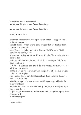
1. Where the Grass Is Greener:
Voluntary Turnover and Wage Premiums
Voluntary Turnover and Wage Premiums
MARLENE KIM*
Standard economic and compensation theories suggest that
voluntary turnover
should decline when a firm pays wages that are higher than
those of its competi-
tors. Turnover behavior in the State of California’s Civil
Service, however, does
not support this prediction. Using a fixed-effects estimator to
control for
job-specific characteristics, I find that the wages California
pays relative to
those of its competitors has little or no effect on turnover. In
addition, estimates
of the elasticity of turnover with respect to alternative wages
indicate that higher
wage rates do not pay for themselves through lower turnover
costs. Instead, the
absolute wage level and wage growth have large effects. In
other words, it
appears that workers are less likely to quit jobs that pay high
wages and have
larger wage increases no matter how their wages compare with
those paid by
other employers.
Introduction

2. A number of theories suggest that voluntary turnover should
decline
when a firm raises its wages relative to what others are paying.
Standard
competitive economic theory predicts that if employers fail to
match the
market wage rate, they will lose their workers to higher-paying
competi-
tors. Because they believe that the wages paid for similar jobs
outside
their firm influence employees’ turnover decisions, human
resource
managers rely on wage surveys to keep their wages competitive
(Mobley,
1982; Milkovich and Newman, 1996).
584
* Department of Labor Studies and Employment Relations,
School of Management and Labor Rela-
tions, Rutgers University. David Card, Bill Dickens, Doug
Kruse, Mark Killingsworth, and Cathy
Weinberger provided exceptionally helpful comments.
INDUSTRIAL RELATIONS, Vol. 38, No. 4 (October 1999). ©
1999 Regents of the University of California
Published by Blackwell Publishers, 350 Main Street, Malden,
MA 02148, USA, and 108 Cowley Road,
Oxford, OX4 1JF, UK.
Job search and efficiency wage theories formalize the
relationship

3. between turnover and comparative wage rates. Models of
employed job
search assume that workers will switch jobs if the expected
discounted
lifetime earnings in an alternative job are greater than the
expected
discounted lifetime earnings in the present job plus the
disutility and
costs of changing jobs. At the margin, these models imply that
the num-
ber of quits will increase if the alternative wage rate increases
relative
to workers’ current expected wage streams (see Burdett, 1978;
Weiss,
1984).
In addition, the turnover version of efficiency wage theory
suggests
that firms with high turnover costs can pay wage premiums in
order to
lower voluntary turnover (Salop, 1979; Summers and Bulow,
1986). If
such firms bear part of the turnover costs, firms can maximize
profits by
increasing wages, since higher costs in wages will be offset by
lower turn-
over costs.1 Firms can therefore set wages to economize on
turnover
costs, with firms having higher turnover costs paying wage
premiums
(see Salop, 1979).
These theories imply that the wage a firm pays relative to its
competi-
tors has a direct effect on turnover and that for some firms this
relation-

4. ship may be cost-effective. Empirically, therefore, we should
observe a
strong negative relationship between relative wages (the wage a
firm
pays relative to its competitors’ wages for the same job) and
voluntary
turnover. However, the empirical findings are mixed. Although
there
is some indication that relative pay among industries and
individuals is
a factor in determining variations in turnover (Mobley, 1982;
Bartel,
1982; Antel, 1988), evidence at the firm level suggests that this
is not
cost-effective.
For example, Leonard (1987) finds a negative correlation
between aver-
age wages and turnover among a cross section of 200 high-
technology
firms; however, the wage premiums are too costly to justify
savings from
lower turnover. Powell et al. (1994) reach similar conclusions
after exam-
ining the wage structure of 205 child care centers. Campbell’s
(1993)
study of more than 5000 firms’ most recent hires also confirms
that turn-
over costs are not sufficient by themselves to account for wages
that
exceed market-clearing levels.2
This article builds on this firm-level research by examining
turnover in
the State of California’s Civil Service (California or California
Service).

5. Voluntary Turnover and Wage Premiums/ 585
1 Turnover costs include direct hiring and training costs and
lost output during this time period.
2 Campbell attributes the cause of his weak findings to long-
term turnover strategies that may not show
up in his cross-sectional study.
The California Service is used as a case study because its data
allow me to
examine a number of different issues that previous studies were
unable to
address. First, because the data are a panel by occupation, I am
able to
control for constant job-specific characteristics that affect
turnover. It is
important to control for job characteristics, since much of
turnover results
from the nature of the job itself (Slichter, 1921; Telly et al.,
1971). Previ-
ous analyses at the firm level (Campbell, 1993; Leonard, 1987)
included
controls for job characteristics (such as blue- and white-collar
composi-
tion of firms and shares of occupation and industry categories);
however,
these may not have adequately controlled for much of the
variation in
turnover among jobs within firms. Their failure to find turnover
cost-effective may have resulted from using average turnover
rates within
firms, which would have masked much of the intrafirm variation

6. in turn-
over at the job level.
Second, because the data include California’s own wage
surveys,
which estimate what its labor competitors pay for the same
occupations, I
am able to control for exact measures of market wages rather
than esti-
mate them by using wage regressions, as does Campbell
(1993).3 These
data allow me to examine how the wages paid by California
relative to
what its labor market competitors pay (calledrelative wages)
affect turn-
over rates within an occupation.
Finally, I am able to examine separately the effects of relative
wages
and absolute wages on turnover. In other words, I am able to
examine
whether turnover responds to wage levels that increase relative
to what
other firms are paying, or whether turnover responds merely to
higher
wages—regardless of how they compare with other firms’ pay.
The next
section describes a simple turnover model and the hypothesized
effects of
wages and labor market conditions. The following section
describes the
data set used to test the model, with the results contained in the
final
section.
A Turnover Model of Efficiency Wages

7. Many models of turnover assume that higher wage rates reduce
turn-
over (see, for example, Flacco and Zeager, 1989), especially
when com-
pared with the alternative wages available (Campbell, 1993;
Salop, 1979;
586 / MARLENE KIM
3 Because predicted wages estimated by wage regressions may
not adequately measure one’s true alter-
native wage rate, measurement error could bias the coefficients
on the alternative wage rates downward,
resulting in Campbell’s (1993) estimates being insignificantly
different from zero. In addition, using the
same regressors to estimate quit rates and alternative wage rates
may have biased the coefficients on the
alternative wages downward as well.
Stiglitz, 1974).4 The model I describe is a simplified version of
Stiglitz
(1974).5 Following Stiglitz (1974), assume that firms produce
outputQ
using a production process that employs capitalK and laborL.
The
production process is described by a production function
Q = F(K, L)
whereFL > 0 andFLL < 0.
For simplicity, assume that labor is homogeneous and that the
capital

8. stock is fixed. Labor costs include training and hiring costs as
well as
wages. Training and hiring costsT include the direct costs of
training and
hiring per worker, such as recruitment, screening, testing, and
orientation,
plus indirect costs, such as lost output when current workers
take time off
from their responsibilities to help newer workers, the costs of
equipment
that is broken, and lost output for new workers while
productivity is
lower. For simplicity, assume thatT is constant. Total training
costs will
depend on the turnover rate of workers, which in turn will
depend on the
wage inside the firmw vis-à-vis the wage rate paid outside the
firmwa.
Turnover also will depend on the unemployment rateu, which
serves as a
proxy for labor market slack. Workers are less likely to quit if
jobs are
scarce, since their chances of obtaining alternative employment
are
smaller (Salop, 1979). The quit rateq is therefore defined as
q = q(w, wa, u) (1)
whereqwa > 0, qw < 0, andqu < 0.
As the wage rate paid by the firm increases, turnover should
decline.
Turnover also should decline when the unemployment rate
increases, but
it should increase when the wages paid by other employers
increase.

9. Voluntary Turnover and Wage Premiums/ 587
4 There are slight differences among these models; however,
most of the general arguments are the
same. Campbell includes the firm’s wage, alternative wage, and
unemployment rate; however, the wages
are separate arguments instead of a ratio. Salop specifies quits
as a function of the ratio of the firm’s wage to
a general measure of labor market tightness, such as the average
wage and nonpecuniary benefits adjusted
for the probability of receiving a job.
5 Stiglitz (1974) has a more complex model, since he estimates
rural and urban wage rates and mobility
between these two sectors. In this article, I reduced this model
to only one sector.
Total labor costs are the following:
w* L = wL + qTL (2)
wherew* is the total labor cost per employee. Setting the price
of output
to unity, the firm’s profits are
F(K, L) − wL − TqL (3)
If the firm chooses its employment level to maximize profits,
FL = w + Tq (4)
The marginal product of labor will equal the wage plus training
costs. If

10. this wagew exceeds the wage that occurs when labor supply
equals labor
demand, unemployment will result.
For a givenL, the firm will minimize the cost per employee:
min(w + qT) (5)
The firm will minimize wage and training costs, taking the
unemployment
rate and other firms’ wages as given. The first-order condition
yields
1 + Tqw = 0 (6a)
or
Tqw = −1 (6b)
The extra wage costs will equal the marginal savings in
turnover costs.6 In
other words, a profit-maximizing firm will continue to increase
wages
588 / MARLENE KIM
6 Allowing for intertemporal profit maximization yields similar
results (see Stiglitz, 1974).
until the last dollar spent is equal to the savings in turnover
costs.
This result is standard for all firm turnover models (see, for
example,
Campbell, 1993). In addition, the greater the training and hiring

11. costsT,
the more likely it is that the efficiency wagew will exceed the
market-
clearing wage rate, resulting in involuntary unemployment.
The Data
To examine the relationship between turnover and relative
wages, I use
unique data from the State of California’s Civil Service. The
California
Service collects market wage data through annual salary
surveys. These
data can be matched to California’s own wage scales and
turnover data
to obtain estimates of wages, market wages, and turnover rates
by occupa-
tion. California’s salary surveys are one of the most
sophisticated surveys
conducted. The Bureau of Labor Statistics established the
survey method-
ology and until the 1980s oversaw the data collection.
Currently, the sur-
vey includes a stratified (by firm size) random sample of 1000
firms in the
State of California. The Bureau of Labor Statistics continues to
collect
data on trades and clerical jobs for the California Service during
its area
wage surveys, while California collects data on professional and
technical
occupations. Since the 1980s, a separate nonprofit agency works
with
businesses and government representatives in the state to
continue these
surveys, using the same methodology as before. An entire year

12. is devoted
to collecting the data, with analysts personally visiting firms
and firms
using job descriptions to match their jobs to those surveyed.
The survey
data estimate market wages for approximately 40 of California’s
4000
detailed occupations.7,8 Although proportionately few
occupations
are surveyed, the California Service surveys those which it
believes are
most affected by external market forces. The surveyed
occupations are
common to many other firms and require less specialized (i.e.,
govern-
ment-only) or firm-specific knowledge. Therefore, these
occupations are
the ones most likely to be influenced by labor market
competition.9 The
Voluntary Turnover and Wage Premiums/ 589
7 The number of occupations surveyed varies by year. In
addition, in some years the sample sizes for
various occupations are too small to compute market averages;
thus the actual number of occupations with
valid market data varies from year to year.
8 Occupationanddetailed occupationare used interchangeably.
They refer to the California Service’s
own detailed occupations, or what are commonly termedjob
titles.
9 Like many government agencies, the California Service
suffers from job title proliferation. Approxi-
mately one-fourth of its job titles contain only one person in

13. them; many are specific to government or
unique to the California Service. Thus many of the 4000 job
titles have no counterpart in other firms that
can be surveyed.
results obtained in this study therefore willoverestimatethe
effect of rela-
tive wages on turnover over all occupations.
For each occupation surveyed, the market data are summarized
into
four measures—the median, average, first, and third quartiles.
The Cali-
fornia Service conducts these wage surveys because it believes
that
recruitment and retention will suffer if it fails to keep up with
the market.
Thus, examining the effects of relative wages on turnover will
confirm
the extent to which retention does suffer.
There are two measures of wages that California pays. The
public wage
scales contain the monthly entry (minimum) rate and the top
(maximum)
rate paid to each occupation (unfortunately, the average wage
paid is
not available). For this analysis, I also calculated the midpoint
rate, the
simple average of the minimum and maximum rates for the
occupation.
The wages used exclude benefit costs; however, because the
same bene-
fits are offered to all employees and remain constant over the

14. time period
examined, omitting benefit costs should not affect the results.10
Data for voluntary turnover in California are from public
records of
voluntary turnover per 100 workers by occupation from July
through
December 1969, 1970, 1974, and 1975 and from January
through June
1970, 1971, 1972, 1974, and 1982–1987.11 Voluntary
turnoversare
defined as voluntary resignations from temporary or permanent
positions
or absences without leaves; retirements are excluded.
The data used in this analysis were constructed as follows: For
each
occupation surveyed, the market wage rates and California’s
wage rates
were collected, as well as the appropriate turnover data. If the
occupation
was surveyed in October, the July through December turnover
rate was
collected. If the occupation was surveyed in July, the January
through
July turnover rate was collected. The total data set includes 494
observa-
tions from approximately 40 occupations over 14 time
periods.12
Although these data allow for excellent measures of market
wages
and turnover for a sample of occupations, they omit other
factors. Work
experience, recent job history (such as recent promotions and
quits), and

15. demographic variables, all of which are associated with
turnover (Antel,
1988; Solnick, 1988; Weiss, 1984; Bartel, 1982; Van den Berg,
1992), are
not available by occupation in California and are therefore
excluded from
590 / MARLENE KIM
10 Benefits for the private sector may fluctuate, however. The
results should be interpreted with this
caution.
11 Data more recent than 1987 were not used because they did
not match the time frame of the salary sur-
veys, and I did not want to contaminate the estimates with
measurement error.
12 Because of some missing data, and because the occupations
surveyed changed during these years, the
total number of observations is 494.
the analysis. In addition, it is possible that the voluntary
turnover rates
may include some “voluntary resignations” that may have been
one step
away from “involuntary separations.”13
Finally, the State of California’s Civil Service may not be a
typical
enterprise. Because it is public, it may not face the same cost-
minimization
constraints as private firms.14 Yet the California Service
believes that turn-

16. over will result if it fails to keep up with the market, and it
collects the
surveyed wage data and sets its wages with this in mind. It
surveys those
occupations which it believes to be the most susceptible to
competitive
market conditions, and it uses surveyed wage measures that it
estimates
to be market wage rates. Thus the results can address the
effectiveness
of California’s own wage policy and whether the California
Service
suffers higher turnover should it fail to pay market wages. In
addition,
although the California Service does not consciously follow an
efficiency
wage strategy, it is still instructive to examine whether paying
wages
that are higher than the market leads to cost savings that justify
wage
premiums.15
Although only one enterprise is examined, it is certainly a major
one.
The California State Civil Service is one of the largest public
employers,
with 150,000 employees, of which 120,000 work full time.
Between
January and June 1987, there were more than 8000 voluntary
turnovers,
of which 6000 were full-time workers. Table 1 displays
voluntary turn-
over rates for the sample of occupations in 1987. As the table
indicates,
voluntary turnover rates vary considerably by occupation. In
addition, the

17. wage rates paid to each occupation relative to what California
claims the
market pays vary over time for each occupation and among
occupations
as well.
A closer examination of the data indicates that wage rates in
the California Service often deviate from market wage rates,
and these
departures are often permanent. In other words, wage rates do
not
Voluntary Turnover and Wage Premiums/ 591
13 On the demand side, these “hidden terminations” may
increase with slack labor markets, if employers
are more willing to reduce their workforce during hard times
when labor is relatively more plentiful. If this
is true, turnover may increase with the unemployment rate,
offsetting the tendency for “true” voluntary
turnover to decline during slack markets. This could explain the
insignificant result I obtain on unemploy-
ment in the first regressions. On the other hand, theoretically,
behavior on the labor supply side may have
the opposite effect: “Hidden terminations” may decline as
unemployment increases, since workers may
decrease shirking or otherwise increase productivity in order to
keep their jobs. This behavior would be
consistent with a negative coefficient on the unemployment
rate.
14 Cost minimization is not essential in order to examine the
turnover behavior of individuals and esti-
mate turnover elasticities with respect to wages, however.
15 This is standard. Previous empirical analyses of the turnover

18. version of efficiency wage theory also
examine firms and industries that do not necessarily follow an
efficiency wage strategy (Leonard, 1987;
Campbell, 1993; Powell et al., 1994).
592 / MARLENE KIM
TABLE 1
VOLUNTARY TURNOVER RATES PER100 WORKERS FOR
THE FIRST 6 MONTHS OF1987
California Service Job Title
Voluntary Turnover
(Per 100 Workers) Relative Wagea
Physical therapist I 11.56 89.97
Security guard 11.29 98.00
Key data operator 9.75 98.50
Food service worker, level B 9.55 86.89
Assistant engineer (various) 9.09 89.54
Electrician, level A 8.93 76.85
Truck driver, level A, B 8.33 75.24
Office assistant II (general), level A 8.06 116.03
Psychologist, clinical 7.79 82.97
Janitor, level A, B 7.69 85.72
Office assistant II (typing), level A, B 7.55 98.32
Delineator 7.08 108.46
Accounting clerk II, level A, B 7.04 99.65
Word processing technician 7.04 87.31
Buyer I, II 6.25 88.82
Laborer 6.25 77.17
Painter, level A 5.97 81.56
Carpenter I, level A 5.75 75.51

19. Secretary 5.65 105.08
Associate engineer (various) 5.26 90.73
Plumber I, level A 4.23 77.00
Programmer II 4.77 86.10
Laundry worker, level B 4.50 108.41
Clinical laboratory technician 3.70 92.59
Stock clerk, level A 2.92 106.45
Associate management analyst 2.83 105.43
X-ray technician 2.78 87.91
Computer operator, level B 2.58 90.93
Pharmacist I 2.54 96.16
Associate budget analyst 2.48 98.95
Stationary engineer, level A, B 2.00 107.09
Accountant trainee 2.00 91.56
Licensed vocational nurse 2.00 87.52
Associate personnel analyst 1.94 101.96
Auto mechanic 1.47 76.65
Mechanical helper 0.00 78.60
NOTE: Voluntary turnover includes voluntary resignations or
absences without leaves. Retirements are excluded.
aMidpoint of California Service’s salary range [(entry level +
top level)/2] divided by median of the surveyed wage rate times
100.
SOURCE: California State Personnel Board.
necessarily converge with the market wages.16 Given the
numerous re-
sources the California Service expended to estimate market
wage rates,
it appears odd that it would not follow them more faithfully.
But the Cal-
ifornia Service, like many employers, followed multiple

20. compensation
goals. Its explicit compensation policy states that besides
paying market
wage rates, it also aims to maintain internal equity in its pay
system, i.e.,
paying jobs it evaluates to require greater skill higher pay
(California
State Personnel Board, 1975). Because the California Service
believed
that changing the relationships dictated by internal equity would
invite
grievances and cause morale problems (Crain, 1986; Atwood,
1986), it
chose not to follow the market “in lock step” if doing so would
disrupt
the internal salary structure (California State Personnel Board,
1975).
The result is that its wage rates often diverge from the market
wages. It
is because of the existence of these deviations that we can
examine
whether turnover responds according to the predictions of
economic
theory.
The Empirical Model
I used the following regression to examine whether turnover
declines if
the wage the California Service pays increases relative to the
wages paid
by other firms for the same occupation. Because the data are a
panel, I
was able to control for job-specific characteristics that
determine turnover
by using a fixed effects (dummy variable) estimator:

21. Turnoveri,t = αi + α2 ln(survey)i,t + α3 ln(wage)i,t
+ α4 (pchwage)i,t + α5 ln(unt) + ei,t (7)
where turnoveri,t is the voluntary turnover rate per 100 workers
for theith
occupation in California in timet, surveyi,t is the surveyed wage
rate for
the ith occupation in timet, wagei,t is California’s wage rate for
theith
occupation in timet, pchwagei,t is the percentage change in
California’s
Voluntary Turnover and Wage Premiums/ 593
16 The following regression,∆ ln wagei,t = β1 + β2 ∆ ln
marketi,t + β3 ∆ ln marketi,t−1 + β4 ln(wagei,t −
marketi,t) + ui,t, showsβ2 = 0.5,β3 = 0.1, andβ4 = −0.0001,
where wagei,t is the wage in the California
Service for occupationi at timet, and marketi,t is the market
wage rate (estimated by the salary survey) for
occupationi at timet. Thus it appears that wage rates change
according to changes in market wage rates,
but they do so incompletely. Moreover, larger gaps between the
market and existing wage rates are not
remedied with larger wage increases, so wages that deviate from
the market do not necessarily catch up
with the market wage rates.
wage rate (in constant dollars) for theith occupation in timet17,
unt is the
unemployment rate in California in timet, αi is the fixed effect
for each
occupation surveyed in California (estimated as a dummy

22. variable), and
ei,t is the error term.
The unemployment rate was included to control for the cyclic
nature of
voluntary turnover due to relatively slack or tight labor markets.
The
coefficient of this variable is expected to be negative. The
dummy vari-
ables for each occupationαi will control for constant
occupation-specific
attributes such as bad working conditions that simply make
some jobs
more desirable than others (Viscusi, 1979; Bartel, 1982). I am
assuming
that these characteristics do not change over the 18-year time
period.18
The coefficient on wagesα3 is expected to be less than zero; the
higher
the wage rate in California, holding the surveyed wage rate
constant, the
lower is the turnover rate in California. Likewise, the higher the
surveyed
wage rate, the higher is the turnover rate, holding California’s
wage rate
constant. Thus I expectα2 > 0.
The change in wage variable is included because workers may
be less
likely to quit their jobs if they recently were awarded real wage
gains,
especially if they form expectations about future wage growth
based on
recent increases (Solnick, 1988). They also may be more likely
to quit

23. their jobs if they receive lower wage increases than they are
accustomed
to receiving. In addition, if information about alternative wage
rates is
imperfect, greater nominal wage increases may fool workers
into thinking
that they are receiving wage rates that are higher than the
market, and it
may take time for workers to learn how their wages compare
with those of
similar employees.
I used four different measures of wages to see if the results
were sensi-
tive to the measurements used. Following the California
Service’s own
convention, I compared the first quartile of the surveyed rates
with the
entry-level rate in California, the third quartile of the surveyed
rates with
the maximum rate in California, and the median and mean
surveyed rates
with the midpoint of California’s rates.19 Table 2 displays the
means of all
the variables used.
594 / MARLENE KIM
17 [(Wagei,t − wagei,t-1/wagei,t−1)] × 100
18 This assumption is plausible given how I constructed the
data set. Many occupations indeed changed
during the 18-year span. However, because of job descriptions
and analysts’ detailed notes regarding the
occupations’ evolution, I was able to determine if the changes
significantly affected the job. If an occupa-

24. tion changed significantly, I simply started a “new” occupation
and discontinued the old one. Because of
such occupation changes and changes in which occupations
were surveyed, few occupations were present
during the entire 18-year period.
19 California compared the first quartile with the entry rate, the
third quartile with the maximum rate, and
the median and mean surveyed rates with its weighted average.
To verify that the fixed-effects model was appropriate rather
than sepa-
rate regressions by occupation, the regression was initially run
separately
for each occupation to examine if the coefficients varied by
occupation
(not shown). Generally, the findings were consistent across
occupations,
indicating that turnover by occupation varies as a shift factor
and not
through interactions with the independent variables. This
confirms that the
fixed-effects model is appropriate.20 Because initial estimates
indicated the
Voluntary Turnover and Wage Premiums/ 595
TABLE 2
VARIABLES AND DEFINITIONS
Variable Definition Mean
Standard
Deviation

25. Quitrates Six-month quitrate per 100 employees 2.56 7.15
Unemployment rate Unemployment rate in California 7.62 1.49
Relative wages
Midpoint/
median
Midpoint of Calif.’s wages/median
of surveyed wages) * 100
91.37 9.51
Midpoint/
average
Midpoint of Calif.’s wages/average
of surveyed wages) * 100
90.65 8.79
Minimum/
1st quartile
Minimum of Calif.’s wages/1st quartile
of surveyed wages) * 100
89.80 9.84
Maximum/
3d quartile
Maximum of Calif.’s wages/3d quartile
of surveyed wages) * 100
92.11 9.82

26. Wage levels
minimum Minimum of Calif.’s monthly wagesa 1719.6 464.81
maximum Maximum of Calif.’s monthly wagesa 2056.1 584.11
midpoint Midpoint of Calif.’s monthly wagesa 1887.8 520.30
ln (minimum) Natural log of the minimum of Calif.’s monthly
wagesa 7.40 0.27
ln (maximum) Natural log of the maximum of Calif.’s monthly
wagesa 7.58 0.27
ln (midpoint) Natural log of the midpoint of Calif.’s monthly
wagesa 7.49 0.27
Surveyed wages
Median Median of surveyed wagesa 2084.56 551.60
Average Average of surveyed wagesa 2149.98 605.53
1st quartile First quartile of surveyed wagesa 1944.34 524.40
3d quartile Third quartile of surveyed wagesa 2241.12 589.25
ln (median) Natural log of median of surveyed wagesa 7.61 0.28
ln (average) Natural log of average of surveyed wagesa 7.63
0.29
ln (1st quartile) Natural log of 1st quartile of surveyed wagesa
7.53 0.28
ln (3d quartile) Natural log of 3d quartile of surveyed wagesa
7.68 0.27
Pchmid Percent change in midpoint of Calif.’s salary
from t − 1 to ta
−0.36 6.59
Pchmin Percent change in minimum of Calif.’s salary
from t − 1 to ta
−0.46 6.64
Pchmax Percent change in maximum of Calif.’s salary
from t − 1 to ta

27. −0.45 6.65
a All wages are in constant (1982–1984) dollars.
20 In addition, the fixed-effects estimator increased the
explained variance by a factor of 10.F tests
indicate that the fixed effects are statistically significant.
presence of first-order serial correlation, the model was
estimated using a
Prais-Winsten (1954) GLS estimator.
Results
Table 3 displays the GLS regression results. As expected,
higher unem-
ployment rates lower turnover. A 10 percent increase in
unemployment
(about a 0.8 point increase in the unemployment rate) reduces
turnover by
0.7 percentage points. Given an average quit rate of 2.6 percent
per six
months, this yields a reduction in the quit rate of 27 percent. In
addition,
the coefficients on the wage variables in California are all
significant.
Increasing wages 10 percent decreases turnover by 1.6 points,
or by 62
percent (−1.6/2.6). Finally, the wage growth variables are also
significant,
596 / MARLENE KIM

28. TABLE 3
TURNOVER, WAGE LEVELS, AND SURVEY WAGESa
(1) (2) (3) (4)
Wage levelb
ln(midpoint) −16.629**
(5.614)
−18.490**
(5.503)
ln(minimum) –15.580**
(5.529)
ln(maximum) –16.736**
(5.567)
Surveyed wage
ln(median) 0.85548
(5.516)
ln(average) 8.5411*
(4.329)
ln(1st quartile) 2.7641
(5.418)
ln(3d quartile) 4.4657
(5.477)
Changes in Calif. Service’s wages
pchmid −0.20698**

29. (0.06555)
−0.23042**
(0.06613)
pchmin −0.19415**
(.06488)
pchmax −0.17075**
(0.06077)
ln(unemployment rate) −7.0419**
(2.600)
−6.6566**
(2.591)
−5.4848*
(2.692)
−7.0049**
(2.682)
Adj R2 0.413391 0.420011 0.407745 0.408086
N 418 418 419 416
* p < 0.05.
** p < 0.01.
a Dependent variable = 6-month voluntary turnover per 100
workers. Standard errors are in parentheses. Fixed-effects
occupa-
tional dummy variables are included. See Table 2 for the
definitions of other variables.
b All wages are in constant (1982–1984) dollars.

30. with a 1 percent increase reducing the quit rate by 0.2
percentage points,
or by 8 percent (−0.2/2.6).
What is surprising is that the coefficients on the surveyed wage
ratesremain
insignificant in three of the four regressions. Moreover, despite
examining a
number of other specifications, I could not find stronger
estimates of these
coefficients. When changes in the surveyed rates are included in
the regres-
sion, for example, the coefficients are all insignificant (see
Table 4). In
Voluntary Turnover and Wage Premiums/ 597
TABLE 4
TURNOVER WITH CHANGES IN SURVEYED WAGESa
(1) (2) (3) (4)
Wage levelb
ln(midpoint) −16.376**
(5.737)
−17.813**
(5.713)
ln(minimum) −16.615**
(5.722)

31. ln(maximum) −16.473**
(5.680)
Surveyed wage
ln(median) −0.41665
(6.155)
ln(average) 6.6046
(5.353)
ln(1st quartile) 4.9484
(6.233)
ln(3d quartile) 2.7399
(6.144)
Changes in Calif. Service’s wages
pchmid −0.2246**
(0.07453)
−0.24533***
(0.07086)
pchmin −0.17082*
(0.07276)
pchmax −0.19152
(0.06812)
Changes in surveyed wages
∆median −0.035395
(0.06878)
∆average 0.02875

32. (0.04649)
∆1st quartile −0.046202
(0.06504)
∆3d quartile 0.043082
(0.06717)
ln(unemployment rate) −7.3976**
(2.689)
−6.5473**
(2.605)
−4.9393**
(2.801)
−7.2317**
(2.717)
Adj R2 0.411910 0.41874 0.4068807 0.4068779
N 417 417 419 414
aDependent variable = 6-month voluntary turnover per 100
workers. Standard errors are in parentheses. Fixed-effects
occupa-
tional dummy variables are included. See Table 2 for the
definitions of other variables.
bAll wages are in constant (1982–1984) dollars.
* p < 0.05
** p < 0.01.
*** p < 0.001.
addition, a number of other specifications were run in order to

33. examine
whetherα2 was underestimated because of using short-term
annual wage
rates instead of long-term wage measures. If turnover responds
to long-term
trends in wage rates, including only annual wages could
underestimate the
impact of relative wages on quit rates. Thus moving averages of
wages
rather than the wage levels were included; however, the
coefficients on mar-
ket wage rates were seldom significant, and when significant,
none came
close to those shown in the second regression in Table 3.21 In
addition, when
long-term changes in turnover were regressed on long-term
changes in wage
rates, the coefficients were insignificant.22
These results suggest that turnover is not affected by what other
employers pay for comparable jobs. Instead, what is important
for turn-
over behavior are the wages one receives and recent wage
changes. In
other words, workers are less likely to quit jobs that pay higher
wages and
that have received larger wage increases, no matter how these
wage rates
compare with those of other employers.
As Leonard (1987) suggests, it is useful to examine the
estimates ofα3
to see if its magnitude supports the efficiency wage theory’s
contention
that it may be cost-effective for firms to increase wages in order
to reduce

34. turnover. Equation (6b) allows me to do so. Usingqw =
[α3/w]/100, α3 =
−16.5, and the average wage of $1888 per month multiplied by
6 for a
6-month estimate ofw, the estimatedqw is equal to
[−16.5/11328]/100, or
−0.000015. I find that paying wage premiums is profitable only
if the
marginal cost of turnover exceeds $66,667 over 6 months,23
which is
much larger than estimates of turnover costs.24 Thus these
results indicate
that quit rates do respond to wage levels, but the magnitude is
insufficient
598 / MARLENE KIM
21 However, if turnover responds to long-term relative wage
rates and these remain constant, turnover
behavior would not change at all, resulting in the low
coefficients on the relative wage variables. This
would occur if relative wage rates are stable in the long run but
vary temporarily in the short run. But rela-
tive wage rates do not follow such a pattern of stable wage rates
in the long run with transitory changes year
to year. In the long run (the time period in the sample), the
wage ratio changed by an average of 9.5 percent
in absolute value, and one-third of the occupations in the
sample had changes in the double digits, with half
of these above 20 percent. Thus it does not appear to be the case
that the year-to-year changes in relative
wage rates are only temporary changes that mask a constant
wage ratio.
22 Ten-year changes in turnover were regressed on 10-year
changes in wage rates. In addition, changes

35. in turnover were regressed on changes in wage rates when using
3-year averages of the final 3 years of data
minus 3-year averages of the first 3 years of data.
23 Given that wage increases affect the wage-change variables
as well as the wage-level variables,
however, the total estimate ofqw may be examined by using
bothα3 andα4. Using−16.5 forα3 and−0.2 for
α4, qw is −0.000032. This means that increasing wages to
reduce turnover is cost-effective if turnover costs
exceed $31,036 over 6 months. This is still not within reason.
24 Campbell (1993) suggests that turnover costs for salaried
employees average $10,000 in 1980, as
estimated by the M and M Association (1980).
to justify wage increases based on the efficiency wage-turnover
theory
when only cost savings from turnover are examined.
Despite examining a variety of different specifications, I could
not find
values ofqw in which higher wages would pay for themselves
through
reduced turnover costs. For example, using wage levels without
a log-
linear form (not shown) produces an estimate ofqw = −0.00006;
this
indicates that wage increases are cost-effective if training costs
exceed
$16,667 over 6 months. Using wage levels rather than the
natural loga-
rithm of the wage produces similar results (qw = −0.00006) if
the wage-

36. change variables are excluded. Using moving averages of wage
rates also
produced smaller estimates ofqw, and regressing long-term
changes of
turnover on long-term changes on wage rates produced
insignificant
results.
One possibility for the low coefficients on the wage variables
may be
due to California Service employees having preferences for
working in
state government or from receiving higher nonpecuniary
benefits, such as
job security, that is unmatched by private-sector employers.
These would
make employees less responsive to changes in relative wage
rates. Yet,
because other studies find low (and even lower) estimates of
quit elastici-
ties among private employers, the unresponsive turnover
behavior does
not seem particular to the California Service.
In fact, overall, these findings confirm those in previous studies
that
although higher wages do reduce quit rates, the elasticity of quit
rates
with respect to wages is too small to justify paying efficiency
wages. My
estimates ofqw are larger than Campbell’s (1993) but smaller
than those
of Leonard (1987) and Powell et al. (1994). Most likely, using
panel data,
omitting demographic characteristics of workers, adding
controls for job-

37. specific characteristics, and using different data and
specifications
account for these differences.
Of course, higher wages may be profitable if firms obtain a
greater
number of job applicants, better labor quality, and a greater
amount of
effort expended per worker. These, plus reduced turnover, could
in com-
bination be sufficient to justify paying higher (efficiency)
wages. Past
research indicates that the number of job applications rather
than tenure
duration may adjust to relative wages (Krueger, 1988).
Unfortunately, I
was unable to examine worker effort and the number of job
applications
in my data set. However, I was able to examine whether labor
quality
adjusted to wage premiums.
I examined this in two ways. First, using CPS data, I examined
the
correlations between the average age and education for state
government
workers in California and a relative wage variable (wages in the
California
Voluntary Turnover and Wage Premiums/ 599
Service divided by the market wage rates). If labor quality
adjusts to wage
premiums, one would expect these correlations to be positive.

38. The correla-
tions between the average education of California state
government work-
ers and relative wages were negative, however, while the
correlations
between the average age of these workers and relative wages
were positive
but insignificantly different from zero. Second, I examined the
correlation
between a labor-quality variable and relative wages. Labor
quality was
estimated from wages predicted from a wage regression on age
and educa-
tion25; these predicted that wages serve as a proxy for labor
quality. If labor
quality increases as a result of higher wage premiums in the
California
Service, one would expect the correlations to be positive.
Correlations
between the predicted wages and the relative wage rates were
negative and
insignificant from zero, however.26 Thus these estimates,
although not
conclusive, suggest that labor quality in the State of California
does not
seem to be the major response to changes in relative wages.
My results differ from previous studies in finding that instead
of relative
wages affecting turnover, wage levels and wage growthwithin a
firm are
important predictors. In other words, workers are less likely to
quit if they
are paid higher wages and receive wage increases, no matter
how these
compare with the wages paid by other employers for similar

39. work. This
implies that wage levels may be important relative to many
alternative uses
of one’s time, only one of which includes working for another
employer. In
addition, the changes in wages have more significant effects on
quit behav-
ior than do the wage levels. Most previous work on turnover
behavior treats
quit rates as a function of the wage level rather than its rate of
change.
600 / MARLENE KIM
25 I did this as follows: First, I ran a simple wage regression
using March CPS data:
wi = B0 + B1agei + B2edi + ui
wherewi is real annual earnings for each full-time year-round
workeri in state government other than
California, agei is the age of each full-time year-round workeri
in state government other than California,
edi is the education level for each full-time year-round workeri
in state government other than California,
andui is the error term. Second, using the estimated
coefficients, I then estimated predicted wages for each
year for California state government workers using CPS data:
where is predicted wages for full-time year-round California
state government workers in yeart, aget is
average age for full-time year-round California state
government workers in yeart, and edt is average edu-
cation level for full-time year-round California state
government workers in yeart. Third, I examined the
correlation between and the average relative wage variable. I
also ran the first regression using local

40. government and private-sector workers in California, but the
correlations between and the average rela-
tive wage variable that I obtained were unchanged.
26 To the extent that the average quality of workers would
change for new hires rather than for the total
workforce, the measurement of predicted wages underestimates
the predicted wages of new hires and
biases the correlations downward.
$w
$w
$w
$ $ $ $w B B Bt t t= + +0 1 2age ed
These results are consistent with Reynolds (1951), who claims
that
workers simply do not change jobs due to better wages paid
elsewhere.
There are many reasons for why voluntary turnover may be
insensitive
to relative wages: Information about wages paid by other
employers is
imperfect, the cost of changing jobs may be prohibitive, fixed
employ-
ment and geographic limitations may inhibit turnover, and
turnover may
simply take time. It seems plausible, as these results suggest,
that workers
have greater knowledge about wages in their own firm—
especially recent
wage changes—than in other firms, causing them to base their

41. decisions
about quitting mainly on recent wage changes in their own firm
and on
how wage levels and wage growth compare historically within
their occu-
pation. Lucas (1972) has proposed such an asymmetrical
information
model for the economy, with agents knowing prices and price
changes in
their own market rather than in the aggregate economy, since
information
is costly. Certainly, further research is warranted to further
investigate
these explanations and their full implications.
Conclusion
Theoretically, voluntary turnover should decline as a firm’s
wages
increase relative to what others are paying. However, evidence
from the
State of California’s Civil Service does not support this. When
control-
ling for occupation-specific job characteristics and using the
California
Service’s own measurements of alternative wages available, I
find that
market wages have little orno effect on voluntary turnover.
However, the
absolutewage level paid for the occupation andwage changesin
that
occupation, rather than therelative wage level, have an effect. In
other
words, for a firm, it does not seem to matter how much one pays
relative
to what other firms pay; rather, what matters are recent wage

42. increases
and whether the job is simply low paid.
Other than the wage level and wage changes, the unemployment
rate
also had a strong effect on turnover. In addition, job-specific
characteris-
tics explained the greatest amount of variation in turnover.
Finally, similar
to previous findings, the results indicate that by itself, the
elasticity of the
quit rate with respect to the wage paid is too small to justify
paying higher
wages in order to reduce turnover costs. These results persist
despite varia-
tions in the model’s specifications.
These results cannot explain why turnover is not more
responsive to
wage rates. It is possible that increasing wages above the
market-clearing
level can still be profit-maximizing if there are productivity
effects
because of increased morale, reduced shirking, or feelings of
gratitude.
Voluntary Turnover and Wage Premiums/ 601
The sum of all these effects could justify paying higher wages.
Further
research is needed to examine these issues.
These results also cannot explain why turnover is not more
responsive

43. to market wage rates. Workers may lack information about
alternative
wages available, face high fixed costs from changing employers
(such as
loss of seniority or pension), or otherwise face significant
mobility costs.
Further research is needed to verify whether these results hold
in the pri-
vate sector. If firms do not suffer the consequences of costly
turnover
should they fail to match their competitors’ salaries, paying
market wage
rates may not bring the benefits of lower turnover that firms
have long
assumed (although, of course, it may be beneficial for
recruitment or
labor quality). This has implications for standard compensation
practices
and the extent to which firms need to invest in salary surveys
and adjust
their salaries according to what their competitors pay. Instead,
what may
be more important for turnover is the growth and level of
paywithin a
firm.
REFERENCES
Antel, John. 1988. “Interrelated Quits: An Empirical Analysis
of the Utility Maximizing Mobility
Hypothesis.”Review of Economics and Statistics70(1):17–22.
Atwood, Jay. 1986. Deposition of Jay Atwood, July 7,
1986.CSEAv. State of California et al.,
C-84-7275 MHP. Federal District Court, San Francisco.

44. Bartel, Ann P. 1982. “Wages, Nonwage Job Characteristics, and
Labor Mobility.”Industrial and
Labor Relations Review35(4):578–89.
Burdett, Kenneth. 1978. “A Theory of Employee Job Search and
Quit Rates.”American Economic
Review68(1):212–20.
California State Personnel Board. 1975. “Overview of the
Salary-Setting Process.” Undated docu-
ment attributed to the mid-1970s.
Campbell Carl M., III. 1993. “Do Firms Pay Efficiency Wages?
Evidence with Data at the Firm
Level.” Journal of Labor Economics11(3):442–70.
Crain, Bruce. 1986. Deposition of Bruce Crain, May 14,
1986.CSEAv. State of California et al.,
C-84-7275 MHP. Federal District Court, San Francisco.
Flacco, Paul R., and Lester A. Zeager. 1989. “The Competitive
Firm with Uncertainty in the Rate of
Labor Turnover.”Southern Economic Journal56(October):457–
66.
Krueger, Alan B. 1988. “The Determinants of Queues for
Federal Jobs.”Industrial and Labor
Relations Review41:4.
Leonard, Jonathan S. 1987. “Carrots and Sticks: Pay,
Supervision, and Turnover.”Journal of
Labor Economics5(4, part 2):S136–52.
Lucas, Robert E., Jr. 1972. “Expectations and the Neutrality of
Money.”Journal of Economic
Theory4(2):103–24.

45. Milkovich, George T., and Jerry M. Newman.
1996.Compensation. Boston: Irwin.
Mobley, William H. 1982.Employee Turnover: Causes,
Consequences, and Control. Menlo Park,
CA: Addision-Wesley.
Powell, Irene, Mark Montgomery, and James Cosgrove. 1994.
“Compensation Structure and
Establishment Quit and Fire Rates.”Industrial
Relations33(2):229–48.
Prais, S., and C. Winsten. 1954. “Trend Estimation and Serial
Correlation.” Discussion paper 383,
Cowles Commission, Chicago.
602 / MARLENE KIM
Reynolds, Lloyd G. 1951.The Structure of Labor Markets. New
York: Harper.
Salop, Steven C. 1979. “A Model of the Natural Rate of
Unemployment.”American Economic
Review69(1):117–25.
Solnick, Loren M. 1988. “Promotions, Pay, Performance
Ratings and Quits.”Eastern Economic
Journal 14(1):51–62.
Summers, Lawrence H., and Jeremy I. Bulow. 1986. “A Theory
of Dual Labor Markets with Appli-
cation to Industrial Policy, Discrimination, and Keynesian
Unemployment.”Journal of

46. Labor Economics4(3, part 1):376–414.
Slichter, Sumner. 1921.The Turnover of Factory Labor. New
York: Appleton and Co.
Stiglitz, Joseph E. 1974. “Alternative Theories of Wage
Determination and Unemployment in
LDC’s: The Labor Turnover Model.”Quarterly Journal of
Economics88(2):194–226.
Telly, Charles S., Wendell L. French, and William G. Scott.
1971. “The Relationship of Inequity to
Turnover Among Hourly Workers.”Administrative Science
Quarterly(June):164–72.
Van den Berg, Gerard J. 1992. “A Structural Dynamic Analysis
of Job Turnover and the Costs
Associated with Moving to Another Job.”The Economic
Journal102(414):1116–33.
Viscusi, W. Kip. 1979.Employment Hazards: An Investigation
of Market Performance. Cambridge,
MA: Harvard University Press.
Weiss, Andrew. 1984. “Determinants of Quit Behavior.”Journal
of Labor Economics2(3):
371–87.
Voluntary Turnover and Wage Premiums/ 603
Copyright of Industrial Relations is the property of Wiley-
Blackwell and its content may not
be copied or emailed to multiple sites or posted to a listserv
without the copyright holder's

47. express written permission. However, users may print,
download, or email articles for
individual use.
THE IMPACT OF MARKET STRUCTURE
ON WAGES, FRINGE BENEFITS, AND TURNOVER
JAMES E. LONG and ALBERT N. LINK*
This paper examines the relationship between labor
compensation and the
structure of the product market, which is measured by the
industry concentra-
tion ratio and by dummy variables for the existence and type of
government
regulation. Unlike previous studies that have estimated the
impact of concen-
tration and regulation on wages or earnings, this study extends
the analysis to
include the effect of market structure on employer-provided
pensions and in-
surance and on voluntary labor turnover. The hypothesis that
product
market power raises labor compensation is supported by
empirical results
indicating that concentration increases wages and fringes but
lowers volun-
tary labor turnover. Regulations that set minimum prices and
restrict entry
raise labor compensation, since wage premiums due to
regulation are not off-
set by lower pensions and insurance or higher turnover. Other
forms of

48. regulation, such as profit regulation in public utilities, are
found to reduce
labor compensation, as evidenced by higher turnover or lower
wages and
fringes, or both.
A LARGE number of studies have exam-ined the impact of
product market
structure on labor earnings. It has been sug-
gested that firms witb market power pay
relatively bigber wages because (1) work-
ers in concentrated industries capture part
of tbe monopoly profits, (2) labor costs in
concentrated industries can be more easily
passed on to consumers, and (3) tbe small
number of firms in concentrated industries
makes it easier for unions to organize and
raise wages. Empirical evidence on tbe
relationsbip between concentration and
•James Long is an associate professor of economics
at Auburn University and Albert Link is a professor of
economics at the University of North Carolina at
Greensboro,
wages is mixed, bowever. Weiss, Masters,
Hawortb and Rasmussen, Asbenfelter and
Jobnson, and Hendricks find tbat con-
centration bas no statistically significant
effect on wages once industrial character-
istics and employee quality are held con-
stant.' In contrast, Dalton and Ford esti-
'Leonard Weiss, "Concentration and Labor Earn-
ings," American Economic Review, Vol, 56, No, 1
(March 1966), pp, 9 6 - 117; Stanley H, Masters, "Wages

49. and Plant Size: An Interindustry Analysis," Review
of Economic? and Statistics, Vol, 51, No, 3 (August
1969), pp, 341-45; Charles T, Haworth and David
W, Rasmussen, "Human Capital and Inter-Industry
Wages in Manufacturing," Review of Economics and
Statistics, Vol, 53, No, 4 (November 1971), pp,376-80;
Orley Ashenfelter and George E, Johnson, "Unionism,
Relative Wages and Labor Quality in U,S, Manu-
facturing Industries," International Economic Re-
Industrial and Labor Relations Review, Vol, 36, No, 2 (January
1983), <
0019-7939/83/3602-0239$01,00
1983 by Cornell University,
239
240 INDUSTRIAL AND LABOR RELATIONS REVIEW
mate that firms in concentrated industries
pay higher wages than competitive firms, a
relationship Haworth and Reuther find
occurring only during cyclical periods of
slack demand and stable prices.^ In sum-
marizing the effects of market structure
on wages, Hendricks points out that the esti-
mated effect of concentration depends on
the control variables and samples used and
on the occupations and time periods exam-
ined.'
To the extent that government regu-
lation can affect the pricing policies and

50. structure of industries, product market
regulation is another potential influence
on labor earnings. For example, by limiting
the entry of firms into the market, regula-
tion may reduce competition and enable
unions to raise wages above the level that
would have existed in the absence of regu-
lation. The resistance of firms to demands
for higher wages may be increased, how-
ever, by regulations that set maximum
prices to insure minimum profits. Hend-
ricks investigates the effect of regulation
on earnings and finds that annual earnings
are lower in regulated industries than in
unregulated manufacturing, a result that
is consistent with Weiss's findings.^ Never-
theless, labor earnings are relatively higher
in industries in which regulatory authori-
ties set minimum prices and restrict entry,
as in trucking and airlines.^ Also, Ehrenberg
view, Vol, 13, No, 3 (October 1972), pp, 488-507;
and Wallace Hendricks, "Regulation and Labor
Earnings," Belt Journal of Economics, Vol, 8, No, 2
(Autumn 1977), pp, 483-96,
2James A, Dalton and E, J, Ford, "Concentration
and Labor Earnings in Manufacturing and Utilities,"
Industrial and Labor Relations Review, Vol, 31, No, 1
(October 1977), pp, 4 5 - 60, and James A, Dalton and
E, J, Ford, "Concentration and Professional Earnings
in Manufacturing," Industrial and Labor Relations
Review, Vol, 31, No, 3 (April 1978), pp, 379-84;
Charles T. Haworth and Carol Jean Reuther, "Indus-
trial Concentration and Interindustry Wage Deter-
mination," Review of Economics and Statistics, Vol,

51. 60, No, 1 (February 1978), pp, 85-95,
'Wallace Hendricks, "Unionism, Oligopoly, and
Rigid Wages," Review of Economics and Statistics,
Vol, 63, No, 2 (May 1981), pp, 198-205,
••Hendricks, "Regulation and Labor Earnings,"
and Weiss, "Concentration and Labor Earnings,"
'See, for example, Hendricks, "Regulation and
Labor Earnings," and Thomas C, Moore, "The Bene-
ficiaries of Trucking Regulation," Journal of Law and
estimates that telephone industry employ-
ees in New York have substantially higher
earnings than other comparable employ-
ees in the state,^
These studies differ in the data bases,
variable definitions, and time periods used,
which complicates any direct comparison
of their results. Yet, one factor is common
to all these studies: they have focused almost
exclusively on wages or nominal earnings.
None, that is, directly considers the influ-
ence of market structure on nonwage com-
pensation such as fringe benefits. Employer
contributions to employee pension and in-
surance plans have grown rapidly in recent
years and now average close to 10 percent of
wages and salaries; in large manufacturing
firms, the percentage is much higher.'
Ideally, for estimating the social costs of
market imperfections, one would want to
know the impact of concentration and
regulation on the total (wage plus non-

52. wage) compensation of workers.
Three empirical issues are therefore con-
sidered in this paper. First, we examine
the impact of market structure on wage
levels, using a data base that has some im-
portant advantages over those used in previ-
ous studies. Second, we analyze the relation-
ship among concentration, regulation,
and employer expenditures on private
pension and insurance funds. And finally,
we estimate the effect of market structure
on labor turnover, holding constant the
influence of concentration and regulation
on wage rates.
Market Structure and Wages
Inadequate control for worker "quality"
can bias the regression estimates of the net
Economics, Vol, 21, No, 2(October 1978), pp, 327-44,
'Ronald G, Ehrenberg, The Regulatory Process
and Labor Earnings (New York: Academic Press,
1979), pp, 69-90,
'For evidence, see James E, Long and Frank A, Scott,
"The Income Tax and Nonwage Compensation,"
Review of Economics and Statistics, Vol, 64, No, 2
(May 1982), pp, 211-19, The 10 percent figure
applies to voluntary rather than legally required
employer contributions, such as OASDHL For a sur-
vey of employee fringe benefits by industry, see Cham-
ber of Commerce of the United States, Employee
Benefits 1980 (Washington, D,C,: Chamber of Com-

53. merce, 1981),
MARKET STRUCTURE AND LABOR COMPENSATION 241
impact of market structure on wages. Eor
this reason, National Longitudinal Survey
(NLS) data have some desirable properties
for wage analyses. Eirst, the NLS contains
data on actual firm-specific work experi-
ence and prior employment history, along
with other important productivity controls
such as educational attainment, duration
of job training, and health status. Second,
the NLS reports individuals' hourly wage
rates, which can be used as dependent vari-
ables in wage equations. Other studies have
resorted to industry averages or have prox-
ied individual wage rates with annual earn-
ings standardized for time worked.* Of
course, the NLS data are not without draw-
backs, namely, the small sample sizes and
narrow age ranges.
We have taken the NLS sample of mature
males (aged forty-five to fifty-nine in 1966)
and estimated wage equations with the
natural logarithm of the hourly wage in
1966 as the dependent variable. The inde-
pendent variables are years of work experi-
ence with the current employer, £XP; ex-
perience squared, EXP^; years of formal
schooling, EDUC; months of job-related
training, TRAIN; a dummy variable equal
to one if health limits working and equal to

54. zero if otherwise, HLTH; a dummy variable
equal to one if married with spouse present
and zero if otherwise, MSP; a dummy vari-
able equal to one if white and zero if other-
wise, WHITE; dummy variables for region,
SOUTH and WEST; the percent of work-
ers in the industry covered by collective bar-
gaining, [/;' the percent of the industry that
'Researchers using the tapes from the 1970 Census
1-1000 Public Use Sample measure annual hours
worked as the product of current weekly hours of work
and weeks worked for the prior year (with both hours
and weeks measured as intervals), a practice tbat
may bias estimates of tbe hourly wage rate.
'The unionization figures refer to the percent of all
production workers in the industry covered by col-
lective bargaining during the period 1968-72, as
estimated from the Expenditures for Employee Com-
pensation Survey administered by the U.S. Bureau of
Labor Statistics. These data can be found in Richard
B. Freeman and James L. Medoff, "New Estimates of
Private Sector Unionism in the United States," Indus-
trial and Labor Relations Review, Vol. 32, No. 2 (Jan-
uary 1979), pp. 143-74.
Ideally, we would like to have information on the
union status of each individual in the sample, but
is employed in plants having 500 or more
employees, LGFIRM; the industry con-
centration ratio, C;'" the interaction be-
tween unionization and concentration,
U'C; and dummy variables for regulated
industries, REG, MAX, MIN, and F^R."

55. Our sample is restricted to 1,514 wage and
salary employees in private, regulated in-
dustries and unregulated manufacturing.
The regression results appear in Table 1.
The basic earnings model. Equation 1,
explains over 40 percent of the variation
in 1966 wages; and all of the control vari-
ables for employee and industry character-
istics are statistically significant with the
expected signs. The coefficients of C and
U'C are highly significant and their signs
indicate that concentration raises wages
although its impact diminishes with union-
ization.'^ A unit increase in concentration
raises wages by .345, .245, .145, and .045
percent at unionization levels of 20, 40, 60,
and 80 percent, respectively." Thus, at a
sucb infonnation is not provided in the census data
used by Weiss and Hendricks or in the NLS data for
the year 1966. Such data are available in the 1971 NLS,
bowever, and we have compared the wage equation
parameters when the industry level of unionization is
replaced by a dummy variable for union membersbip
(more correctly, coverage of tbe individual by a collec-
tive bargaining contract). These results indicate that
the coefficients of the concentration and regulation
variables do notvary witb the measure of unionization.
'"Concentration estimates for the industry categories
in the NLS sample were kindly provided by Wallace
Hendricks.
"M/IX denotes industries in which maximum prices
are regulated (telephone, electricity, gas and steam,

56. water); MIN denotes industries in which minimum
prices are regulated and also entry is restricted (air
transportation, trucking); and VAR denotes all otber
regulated industries (railroad, bus, taxicab, ware-
housing, water transportation, services incidental to
transportation, radio and television, and sanitary).
REG includes all of these regulated industries. See
Hendricks, "Regulation and Labor Earnings," pp.
485-87, for a discussion of the primary regulatory
authority and its powers in various industries.
'2A negative relationship between wages and [/• C
was also found by Weiss, "Concentration and Labor
Earnings"; Frederic M. Sherer, Industrial Market
Structure and Economic Performance, 2d ed. (Chicago:
Rand McNally, 1980), p. 359; and Hendricks, "Union-
ism, Oligopoly, and Rigid Wages."
I'These estimates are obtained by evaluating the
expression
3 WAGE/ dC = .00445 - .00005 U.
242 INDUSTRIAL AND LABOR RELATIONS REVIEW
Table L Regression Analyses of the Effect of
Concentration and Regulation on Wage
Rates, 1966.
(^-values in parentheses)
Variables
C

57. u.c
REG
MAX
MIN
VAR
U
LGFIRM
EXP
EXP^
MSP
EDUC
TRAIN
SOUTH
WEST
WHITE
Constant
R
̂
F-level

58. N
Equation 1
,00445**
(3,06)
- ,00005*
(-2,41)
- ,01804
(-,60)
—
,00436**
(3,39)
,33277*
(2,36)
,01216**
(4,72)
- ,00012
(-1,78)
,09119**
(2,92)
,04275**
(14,72)
,00204**
(3,50)

59. -,14971**
(-6,89)
,14187**
(5,25)
,15275**
(6,90)
4,57168**
(50,50)
,4250
85,52
1514
Equation 2
,00492**
(3,42)
-,00003
(-1,72)
—
-,00211
( - , 0 4 )
,14863**
(3,24)
-,16692**

60. (-4,27)
,00349**
(2,62)
,2393
(1,71)
,01197**
(4,69)
-,00011
(-1,57)
,09882**
(3,19)
,04156**
(14,45)
,00208**
(3,62)
-,14113**
(-6,55)
,14673**
(5,49)
,14882**
(6,77)
4,57487**
(50,86)
,4395

61. 78,29
1514
unionization level of 70 percent (the sample
mean), wages in high-concentration indus-
tries (C equals 70 percent) are 4.75 percent
higher than wages in low-concentration in-
dustries (C equals 20 percent). In contrast,
the wage differential between high-union-
ization {U equals 70 percent) and low-
unionization industries {U equals 20
percent) is 8.8 percent at the mean con-
centration level of 52 percent.
In Equation 2, the single dummy variable
for industry regulation {REG) is replaced
by separate variables for the specific type of
regulation {MAX, MIN, and VAR). The
estimated coefficients of the concentration
terms now imply a much larger impact of
market power on wages—about a 14 percent
wage differential between high- and low-
concentration industries. Controlling for
the specific type of industry regulation is
thus important in estimating the net impact
of concentration on wages, as well as in
estimating the union wage effect (which
increases to 9.6 percent in Equation 2).
The finding that concentration raises
wages is very robust and does not depend
on cyclical factors such as high unemploy-
ment and stable prices, as suggested by
Haworth and Reuther, or on concentra-

62. tion's being less than some critical value,
as estimated by Dalton and Ford.'* This
conclusion (as well as those of previous
studies) should he tempered, however, hy
the recognized weaknesses of concentration
ratios, including the fact that the industry
definitions used in their measurement are
arbitrary and do not necessarily conform
*Significant at the ,05 level in a two-tailed test,
**Significanl at the ,01 level in a two-tailed test.
''Haworth and Reuther, in "Industrial Concentra-
tion and Interindustry Wage Determination," find
the concentration impact on wages to be positive and
significant only during a recessionary period. The
year 1966 was one of low unemployment (2,9 percent).
When our wage equations were estimated with NLS
data for 1971, a year of high unemployment (5,0 per-
cent), the impacts of high concentration and MIN-
regulation on wages were similar to those reported in
Table 1 and equally significant,
Dalton and Ford, in "Concentration and Labor
Earnings," estimate that increases in concentration
above the 50 percent level do not affect manufac-
turing wages. We find that estimating the wage equa-
tions with concentration-squared terms leaves the
estimated wage differentials between high- and low-
concentration industries virtually unchanged.
MARKET STRUCTURE AND LABOR COMPENSATION 243
to economic markets and also the fact that

63. no information is provided about the mar-
ket shares of individual firms.
The estimated coefficient of REG in
Equation 1 is not statistically different
from zero, wbicb indicates that wages do not
differ between regulated industries and un-
regulated manufacturing, once human
capital, location, and industry character-
istics are held constant. The estimates in
Equation 2 substantiate Hendricks's hy-
pothesis that a single dummy variable mis-
represents the wage impact of industry
regulation.'5 Regulation has no effect, for
example, on wages in utility industries in
which maximum prices {MAX) are set and
entry is restricted, such as the telephone,
electricity, gas and steam, and water indus-
tries. This finding suggests that the impact
on labor costs of "cost price-through"
utility pricing schemes is offset by the in-
flexibility of rate changes due to regulatory
lags.'^
Setting minimum prices (MIN) and con-
trolling entry into tbe market, on the other
hand, raises wages by about 15 percent,
suggesting tbat union power in air trans-
portation and trucking is increased by regu-
lations that reduce competition from non-
union labor. Finally, wages are nearly 17
percent lower in railroads, local passenger
transit, warehousing, radio and television,
and other industries in wbich regulatory
practices are more varied {VAR) and have
not altered market structure and pricing

64. policies in ways tbat might increase union
power.
Assigning the degree and type of regula-
tion to an industry also involves some
arbitrary judgments that qualify the infer-
ences drawn from the coefficients of the
regulation variables. In addition, a problem
in interpreting the coefficient of MIN is
that air transportation and trucking are in-
dustries characterized by spatial production
limitations that act to curb the entry of new
firms outside the union's jurisdiction. In
long-line trucking, for example, a union
firmly established in a few key cities within
a region will be protected from nonunion
competition because new entrants must
almost always operate in the same key
cities. Levinson argues that these spatial
limitations of production, rather than the
control of entry by regulatory authorities,
are responsible for the Teamsters' success
in raising wages.^'
In this paper, we are unable to determine
which entry barrier—spatial production
limitations or regulation—is more im-
portant in raising wages in air transporta-
tion and trucking.'^ Nonetheless, we be-
lieve it is important to include the regula-
tion variables in the wage equation, if for no
other reason than to serve as controls for
estimating the wage impact of concentra-
tion.

65. Since the earnings model includes a num-
ber of control variables for worker quality
and industry characteristics, the findings in
Table 1 suggest tbat employees in high-
concentration and M/N-regulation indus-
tries receive economic rent in the form of
wage premiums. Tbe correct measure for
determining whether workers receive eco-
nomic rent, however, is total labor compen-
sation, wbicb equals wages and salaries
plus sucb nonwage compensation as em-
ployer-provided fringe benefits (pensions
and health insurance), job satisfaction, and
employment stability. The impact of mar-
ket structure on nonwage compensation is
'^Hendricks, "Regulation and Labor Earnings."
"For additional discussion, ̂ see Ehrenberg, The
Regulatory Process and Labor Earnings, pp. 11-12.
"Harold M. Levinson, "Unionism, Concentration,
and Wage Changes: Toward A tJnified Theory,"
Industrial and Labor Relations Review, Vol. 20, No.
2 (January 1967), pp. 198- 205.
'*Both theory and empirical evidence suggest that
the latter effect may dominate. Moore, "The Bene-
ficiaries of Trucking Regulation," argues that the
operating-ratio regulation in trucking tends to in-
crease labor costs, aside from any additional union
strength due to reduced competition from nonunion
drivers. Empirically, the annual growth in hourly
earnings in trucking has slowed considerably since
1977, relative to earnings growth during earlier years
and relative to manufacturing wage increases since

66. 1977. Entry into trucking has been less restricted since
1977, particularly for short-haul carriers, and de-
regulation policies have been gaining support. Since
there is little reason to expect that spatial production
limitations have changed radically since 1977, the
relatively slower wage growth in trucking may reflect
the influence of greater competition.
244 INDUSTRIAL AND LABOR RELATIONS REVIEW
examined in the following sections of the
paper.
Market Structure and Fringe Benefits
Data on one form of nonwage compensa-
tion—voluntary employer contributions for
pension and profit-sharing plans and for
group health and life insurance—can be
derived from U.S. Department of Commerce
estimates of employee compensation by
industry.'8 In estimating the relationship
between market structure and employer
expenditures on these fringe benefits, it is
important to control for those determinants
of fringe benefits that correlate with con-
centration and regulation. The variables
expected to affect fringes have already been
discussed in detail elsewhere, so only a brief
description of the model is presented here.^"
Fringe benefits should vary positively
with total employee compensation because
of tbe positive income elasticity of demand

67. for fringes and the positive tax-rate elas-
ticity that results from the preferential tax
treatment of fringe benefits.^' Unionization
is thought to have a positive effect on fringe
benefits, since union leaders can inform
their members of the tax advantages of
fringe benefits and of the cost savings of
group insurance and since employee prefer-
"U.S. Department of Commerce, Survey of Current
Business, Vol. 59, No. 7 (July 1979), pp. 54-55. Vol-
untary employer contributions for pensions and insur-
ance were estimated by first subtracting wages and
salaries from total employee compensation and then
subtracting tbe legally required employer con-
tributions to OASDHI. OASDHI payments by industry
were calculated as (.mOb)(WAGE)(FTE) for WAGE >
517,700 or ($1,071) (FTE) for WAGE <' $17,700, where
WA GE is average annual wage and salary earnings per
full-time employee and FTE is total industry full-time
employment.
2»See Robert G. Rice, "Skill, Earnings, and the
Growth of Wage Supplements," American Economic
Review, Vol. 56, No. 2 (May 1966), pp. 583-93;
Bevars Mabry, "The Economics of Fringe Benefits,"
Industrial Relations, Vol. 12, No. 1 (February 1973),
pp. 9 5 - 106; Richard B. Freeman, "Tbe Effect of
Unionism on Fringe Benefits," Industrial and Labor
Relations Review, Vol. 34, No. 4 (July 1981), pp.
489-509; and Long and Scott, "The Income Tax
and Nonwage Compensation."
2'See John S. Nolan, "Taxation of Fringe Benefits,"
National Tax Journal, Vol. 33, No. 3 (September
1977), pp. 359-68.

68. ences for fringe benefits can be directly
transmitted to management by collective
bargaining. Because of rate differentials be-
tween group and individual health or life
insurance policies, fringe benefits should
vary directly with firm size, assuming the
demand for group insurance is price-elastic.
Employers may have a preference for certain
types of fringe benefits that reduce labor
turnover, sucb as nonvesting pension plans
or paid vacations whose length increases
with tenure. These kinds of fringe benefits
are most likely to be offered when turnover
costs are high, which is the case if much of
employees' human capital is firm-specific.
The impact of concentration and regula-
tion on fringe benefits is obtained by esti-
mating the equation:
(1) FBi =a +bC, +cRi + dXi ,
where FB, is annual voluntary employer
expenditures in 1978 on pensions, profit
sharing, and insurance, measured as dollars
per full-time employee; C; is the industry
concentration ratio; /?, consists of dummy
variables indicating the existence and type
of regulation, as defined earlier; and the
vector X, includes the control variables
TOTCOMP (average annual total com-
pensation per employee), FIRMSZ (average
firm size), KLRA TIO (the ratio of capital to
labor), U (the percent of industry employees
covered by collective bargaining), and U'C
(an interaction between unionization and
concentration). Data for these variables are

69. available for twenty-eight two- and three-
digit industries, which include manufac-
turing, transportation, communication,
and public utilities.^^ The ordinary least
'^Concentration ratios for two-digit manufactur-
ing industries came from William G. Shepherd, The
Economics of Industrial Organization (Englewood
Cliffs, N.J.: Prentice-Hall, 1979), p. 202. Concentra-
tion data for regulated industries were provided by
Wallace Hendricks. For two industries (local and
inter-urban passenger transit and trucking and ware-
housing), it was necessary to average his data for cen-
sus industries (using industry employment as weights)
to match the Department of Commerce industry defi-
nitions. Average firm size was measured as the num-
ber of employees per establisbment in 1977, as re-
ported in the U.S. Bureau of Census, County Business
Pattems 1977, United States Summary, CBP-79-1
MARKET STRUCTURE AND LABOR COMPENSATION 245
square estimates of tbe model are reported in
Table 2.2'
Table 2. Regression Analyses of tbe Effect of
C o n c e n t r a t i o n and Regulation on
Employer Contributions for Pensions and
Group Insurance, 1978.
(^-values in parentheses)
Variables

70. C
u«c
REG
MAX
MIN
VAR
U
TOTCOMP
FIRMSZ
KLRATIO
Constanl
R
̂
F-level
N
Equation 1
-31.189*
(-2.55)
.854**
(3.90)

71. - 626.523
(-1.67)
—
—
—
-11.516
(-.81)
.085*
(2.44)
4.205
(1.92)
129.576**
(5.72)
317.782
(.51)
.936
41.51
28
Equation 2
- 19.804
(-1.48)
.653*

72. (2.64)
—
-230.861
(-.37)
-401.641
(-1.03)
-986.703*
(-2.09)
-.086
(-.01)
.072
(1.99)
3.904
(1.75)
124.217**
(5.24)
21.618
(.03)
.946
35.26
28
*Significant at the .05 level in a two-tailed test.
**Significatit at the .01 level in a two-tailed test.

73. (Washington, D.C: GPO, 1979), pp. 1-2. TOT-
COMP and KLRATIO (which is proxied by the ratio
of corporate capital consumption allowances to in-
dustry employment) came from the LI.S. Department
of Gommerce. Survey of Current Business, Vol. 59,
No. 7 (July 1979), pp. 54, 55, and 60. tjnionizationdata
are from Freeman and Medoff, "New Estimates of
Private Sector Llnionism in the LInited States."
"Freeman, in "The Effect of Unionism on Fringe
Benefits," p. 498, has pointed out that Equation
Tbe concentration terms are bigbly sig-
nificant in Equation 1, wbich includes only
tbe single regulation variable. Tbe co-
efficients of C and U'C indicate tbat product
market power raises fringe benefits, once
unionization exceeds 37 percent.̂ ^ Tbe
marginal effects of concentration on fringe
benefits are - 14, +3, +20, and +37 dollars at
unionization levels of 20, 40, 60, and 80
percent, respectively. At a unionization level
of 44 percent (tbe sample mean), tberefore,
pension and insurance contributions are
|320 bigber in bigb-concentration (C
equals 70 percent) tban in low-concentra-
tion (C equals 20 percent) industries. Wben
tbe tbree regulation variables are included
in place of REG, as in Equation 2, tbe abso-
lute values of tbe concentration coefficients
are diminisbed; but tbe U'C term,bow-
ever, remains positive and bigbly signifi-
cant. Tbe estimates indicate tbat market
power raises fringe benefits at unionization
levels above 31 percent; at tbe mean level,

74. employer contributions for pensions and in-
surance are $425 bigber in bigb- tban in
low-concentration industries. Tbe impact
of concentration on fringe benefits is tbus
mucb smaller tban tbe $1,575 effect due to
unionization.^*
1 is subject to simultaneity bias since TOTCOMP
includes voluntary employer contributions for fringe
benefits along with wages and salaries plus legally
required supplements. Gorrecting for this problem, as
he suggests, does not appreciably change our estimates
of the impact of concentration and regulation on
fringe benefits. Gonsequently, the corrected estimates
are not reported in the text.
2*Note that the positive and significant coefficient
of U'C in Table 2 contrasts with that observed in
Table I and in other wage studies. Together, these re-
sults indicate that in highly concentrated industries,
increased unionization raises the sbare of total com-
pensation allocated to fringe benefits—a finding
consistent with the theory and evidence presented by
Freeman, "Tbe Effect of Unionism on Fringe Bene-
fits." The tax savings from fringe benefits increase
witb concentration; and unions can inform members
of the advantages of fringes and make worker prefer-
ences concerning the compensation mix known to
management.
2*Tbis estimate assumes a concentration level of 49
percent (the sample mean) and a unionization differ-
ential of 50 percent (for example, U equals 70 percent
relative to U equals 20 percent).

75. 246 INDUSTRIAL AND LABOR RELATIONS REVIEW
When measured by a single variable,
industry regulation reduces fringe benefits
by $627, although the statistical significance
of REG is marginal. Equation 2 suggests
that the negative effect of regulation on
fringes should not be attributed to all types
of regulation. Pension and insurance con-
tributions are relatively lower (by |987)
only under VAR-type regulation, in which
authorities do not consistently restrict entry
or set minimum and maximum prices.
We know of no previous studies that have
related fringe benefit expenditures to con-
centration and regulation; consequently,
there are no benchmarks against which our
estimates can be compared. Moreover, since
we use aggregate industry data, our con-
clusions should be regarded as tentative. In
the next section we propose an alternative
test to determine the influence of concen-
tration and regulation on nonwage com-
pensation.
Market Structure and Labor Turnover
An alternative method for estimating the
effect of market structure on nonwage com-
pensation is derived from the assumption
that, other things equal, individuals will
quit their present jobs if they perceive that
an alternative job offers a net advantage.
If concentration or regulation generates

76. positive (negative) economic rent in terms
of higher (lower) wage or nonwage returns,
workers in concentrated or regulated indus-
tries will therefore be less (more) likely to
quit and move to other jobs than workers in
competitive industries. Interindustry turn-
over differentials not resulting from wage
differences among concentrated, regulated,
and competitive industries can thus be as-
sumed to result from differences in nonwage
compensation.26
2'A number of recent studies have used turnover
data to analyze nonwage differentials by race and
union status. For example, see Duane E, Leigh,
"Unions and Nonwage Racial Discrimination,"
Industrial and Labor Relations Review, Vol, 32, No,
4 (July 1979), pp, 439-50; and Richard B, Freeman,
"The Effects of Unionism on Worker Attachment to
Firms," Journal of Labor Research, Vol, 1, No, 1
(Spring 1980), pp, 29-62, James E, Long has used
quit behavior to estimate whether government workers
The impact of market structure on labor
turnover has not been extensively re-
searched, Hendricks indicates that regulated
industries offer more stable employment
than manufacturing, and Ehrenberg reports
that quit rates are much lower for New York
Telephone employees than for workers in
manufacturing industries. Nevertheless,
neither conclusion is supported by multi-
variate analysis that controls for nonregula-
tion variables that influence turnover.^'
Other empirical studies have found a

77. significant, negative relationship between
concentration and the industry's average
annual quit rate. Burton and Parker suggest
that quits are inversely related to concentra-
tion because (1) the relatively high profits of
concentrated industries may allow those
firms to use labor in an inefficient (in other
words, X-efficient) manner, which may be a
characteristic of employment that is attrac-
tive to workers; (2) the fewness of firms raises
the probability of collusive no-raiding
agreements as well as reduces alternatives
for intra-industry mobility; and (3) fringe
benefits may be higher in concentrated
industries.28 Parsons argues that entrance
into high-concentration, high-wage indus-
tries generally requires investments by the
worker, which may diminish the tendency
to quit.29
These concentration-turnover findings
came from regression models of the form
(2) QR= )So+ fi,W+ I3,A + ^ , 2 ,
where QR is the industry quit rate, W is the
current wage, A represents alternative job
possibilities, and Z is a vector of other deter-
are overpaid relative to private sector employees, in
"Are Government Workers Overpaid? Alternative
Evidence," Journal of Human Resources, Vol, 17,
No, 1 (Winter 1982), pp, 123-31,
"Hendricks, "Regulation and Labor Earnings," p,
492; Ehrenberg, The Regulatory Process and Labor

78. Earnings, pp, 108- 110,
28John F, Burton and John E, Parker, "Interindustry
Variations in Voluntary Labor Mobility," Industrial
and Labor Relations Review, Vol, 22, No, 2 (January
1969), pp, 199-216,
"Donald O, Parsons, "Specific Human Capital: An
Application to Quit Rates and Layoff Rates," Journal
of Political Economy, Vol, 80, No, 5 (November/
December 1972), pp, 1120-43,
MARKET STRUCTURE AND LABOR COMPENSATION 247
minants of the quit rate (such as pensions,
race, gender, and concentration). This
specification can be criticized on two
grounds. First, using industry aggregates as
the units of observation introduces a simul-
taneous-equation bias because it is ambigu-
ous whether Equation 2 is a supply or de-
mand relationship,'" With individual work-
ers as the unit of observation, however.
Equation 2 can be treated as a supply rela-
tionship, because the compensation levels
facing individual workers are exogenous to
them, A second statistical problem is the
inclusion of wages as an explanatory vari-
able, Flanagan argues that this introduces
multicoUinearity (since wages may be re-
lated to race, gender, concentration, and
other explanatory variables) and a simul-
taneity problem (employers may pay lower
wages to workers more likely to quit, for

79. example)."
With these problems in mind, we esti-
mate the relationship between market
structure and voluntary turnover using the
following model specified by Flanagan:'^
(3) a = /8o+ J8,(M .̂- - M )̂+ /̂ 2 2 , .
where Q, is the quit behavior of the indi-
vidual, Wi is the individual's current wage,
W is the mean market wage for workers with
similar human capital and wage-related
characteristics, and Z, contains other deter-
minants of quit behavior. The probability
of quitting the current employer is assumed,
other things equal, to increase as the differ-
ence between the actual current wage and
the "potential" market wage (hereafter,
RESID) decreases. For our analysis, the
vector Z includes dummy variables indicat-
ing whether the current employer is in a
regulated industry {REG, MAX, MIN, or
VAR); the concentration ratio (C) in the
individual's current (three-digit census)
industry; unionization {UNION) in the
'"For further discussion, see Schiller and Weiss,
"The Impact of Private Pensions on Firm Attach-
ment," p, 379,
"Robert J, Flanagan, "Discrimination Theory,
Labor Turnover, and Racial Unemployment Differ-
entials," Journal of Human Resources, Vol, 13, No,
2 (Spring 1978), pp, 187-207,

80. "Ibid,
current industry; years of work experience
with the current employer {TENURE);
and dummy variables for married with
spouse present {MSP) and race {WHITE).
If high concentration and regulation gen-
erate positive (negative) economic rents, the
coefficients of C and the regulation vari-
ables are expected to be negative (positive)
and statistically significant. Since the effects
of concentration and regulation on the cur-
rent wage will be held constant by the
RESID term, negative coefficients on the
market-structure variables will indicate that
concentration and regulation raise non-
wage compensation. From previous studies,
we expect the quit probability to vary in-
versely with TENURE, MSP, and UNION
and directly with WHITE.
Turnover data for individual workers
and for the explanatory variables required to
estimate Equation 3 were obtained from the
National Longitudinal Surveys (NLS) of
middle-aged men (aged forty-five to fifty-
nine)," In the NLS, individuals are asked
to compare their employers at two consecu-
tive survey dates and to indicate whether
any change in employers is due to a volun-
tary quit or to layoff or dismissal. In the
sample of middle-aged males, comparison
data on employers are reported for the years
1966-67, 1967-69, 1969-71, and 1971-
73. Labor turnover can thus be measured
as a binary variable taking a value of one if a

81. worker quits his or her job in one year and
has a different employer in a later year, and
taking value of zero if that worker does not
change or involuntarily changes employers.
Combining data for the four intervals pro-
vides a sample of 4,408 observations, in-
cluding 177 instances of job quitting.
The variable RESID is calculated by
subtracting individual workers' "potential"
(predicted) wage from their actual wage at
the beginning of a time interval. The pre-
dicted wage is based on the coefficients
from a market wage equation, using the
natural logarithm of the hourly wage as
the dependent variable and including the
following explanatory variables: years of
"Data sources for the concentration and unioniza-
tion variables may be found in footnotes 10 and 11
above.
248 INDUSTRIAL AND LABOR RELATIONS REVIEW
schooling; tenure and its square; unioniza-
tion; months of job-related training; and
dummy variables for health, marital status,
race, and geographic region. Since the
turnover observations are pooled by time
intervals, four separate wage equations are
estimated. The wage equation samples are
restricted to private wage and salary em-
ployees in manufacturing and regulated
industries.

82. Our estimates of the impact of market
structure on voluntary turnover are reported
in Table 3 . " Since the dependent variable
is dichotomous, the quit equations are esti-
mated with probit analysis. The coefficient
of concentration is negative and highly
significant in both equations, indicating
that the probability of quitting decreases
as concentration rises. In contrast, the co-
efficients of regulation (REG) are positive,
which indicates that individuals employed
in regulated industries are more likely to
voluntarily change employers than workers
in unregulated manufacturing. Equation 2
reveals, however, that the positive impact of
regulation on turnover is statistically sig-
nificant only for MAX- and VAR-iype
regulation.
The coefficients of the remaining vari-
ables carry the predicted signs, and RESID,
TENURE, and UNION are highly signifi-
cant. Since including RESID in the quit
equation holds constant any "wage differ-
ential" incentive for changing employers,
the negative coefficient of C in Table 3 sug-
gests that quitting decreases as concentra-
tion rises because nonwage compensation
is greater in highly concentrated industries
than in competitive industries. This find-
ing is consistent with the estimates in Table
2, which indicate that employer expendi-
tures on pensions and insurance increase
with concentration. The results in Tables 2
and 3 suggest that workers in VAR-regula-

83. . Probit Analyses of the Effect of Con-
centration and Regulation on Voluntary
Labor Turnover, 1966-73.
(asymptotic lvalues in parentheses)
'*To determine whether our estimates are biased by
pooling different time intervals, we included the
national rate of unemployment during the first year of
each interval as a crude measure of labor market
conditions. This variable was never statistically sig-
nificant and its inclusion had no effect on the market
structure coefficients; it was therefore dropped from
the equation.
Variables
C
REG
MAX
MIN
VAR
RESID
TENURE
UNION
MSP

84. WHITE
Constant
- 2 X log
likelihood
ratio
N
Equation I
- .0068**
(-3.13)
.3337**
(3.11)
-.2014*
(-2.10)
- .0489**
( - 10.64)
- .0059**
(-2.67)
-.1484
(-1.24)
.0973
(1.13)
-.4761**
(-2.74)

85. 231.36
4408
Equolion 2
-.0111**
(-3.64)
—
.7398**
(2.57)
.0721
(.42)
.5687**
(3.37)
-.1785
(-1.83)
- .0493**
(-10.64)
- .0048*
(-2.06)
-.1545
(-1.24)
.1250
(1.43)

86. - ,3767*
( - 2.08)
235.95
4408
*Significant at the .05 level in a two-tailed test.
**Significant at the .01 level in a two-tailed test.
tion industries are relatively more likely to
quit because they receive lower fringe bene-
fits than comparable workers in other regu-
lated industries and manufacturing. The
insignificance of the MIN terms in Tables 2
and 3 implies that setting minimum prices
and restricting market entry raises wages
but does not affect other kinds of labor com-
pensation. The coefficients oiMAX suggest
that regulation in the utility industries re-
duces certain kinds of nonwage compensa-
tion (other than pension and insurance
MARKET STRUCTURE AND LABOR COMPENSATION 249
payments) and, other things equal, results
in higher labor turnover.'^
Summary and Implications
Previous studies of the effect of con-
centration and industry regulation on labor
compensation have focused predominantly
on wages or earnings while ignoring fringe

87. benefits and other kinds of nonwage com-
pensation. Consequently, the implications
of those studies regarding the impact of
market structure on total labor earnings
must be considered tentative. In this study,
we have empirically examined the effect of
concentration and regulation on labor
compensation by estimating the deter-
minants of hourly wages, fringe benefits in
the form of employer contributions to pen-
sion and insurance plans, and voluntary
labor turnover. The regression results reveal
a positive and highly significant relation-
ship between concentration and both wages
and fringes, and a significant negative rela-
tionship between concentration and job
quitting. These findings are highly con-
sistent with the hypothesis that, other things
equal, labor compensation is relatively
higher in concentrated industries than in
more competitive ones. Thus, it is rather
ironic that certain members of Congress
with close ties to organized labor, notably
Senator Edward M. Kennedy, have sup-
ported legislation intended to reduce in-
dustrial concentration in the United
States.56
'^These kinds of nonwage compensation could
include vacation and sick-leave pay, bonuses, over-
time premiums, contributions to savings plans,
holiday funds, employee education funds, job security,
and job satisfaction. For information on the various
kinds of fringe benefits, see Chamber of Commerce
of the United States, Employee Benefits 1980; and
Freeman, "The Effect of Unionism on Fringe Bene-

88. fits." Freeman's data (p. 496) indicate that employer
contributions for pensions and insurance make up
only about 36 percent of measurable voluntary fringe
benefits.
"Opening statement of Edward M. Kennedy in U.S.
Congress, Senate, Committeeon the Judiciary, Mergers
and Economic Concentration, Part 1, Hearings before
the Subcommittee on Antitrust, Monopoly, and
Business Rights (Washington, D.C: GPO, 1979). For
additional discussion, see A. F. Ehrbar, "Bigness
Industry regulations that set minimum
prices and restrict market entry, as in air-
lines and trucking, are estimated to raise
labor compensation by means of increasing
hourly wages. This result implies that the
opposition to deregulation on the part of
the Air Line Pilots Association and the
Teamsters has been well founded. The rela-
tively higher incidence of job quitting
among workers in the utility industries
(telephone, electricity, gas, and water)
suggests that profit regulation through
the imposition of maximum prices reduces
labor compensation. Stronger evidence that
certain kinds of regulation may decrease
labor earnings is contained in the finding
that in the remaining regulated industries,
both wages and fringe benefits are relatively
lower, wbereas voluntary labor turnover is
relatively higher.
The implications of this study for public
policies designed to deconcentrate or de-
regulate industries depend on two issues.

89. First, has labor quality adequately been beld
constant in the empirical analyses, so that
compensation differentials reflect eco-
nomic rent rather than payment for some
productivity factor? Second, do the empiri-
cal findings for mature men apply to other
groups of workers as well? If we assume
that the relatively higher labor compensa-
tion in concentrated and M/N-regulated
industries constitutes economic rent en-
joyed by the average worker in those indus-
tries, then our findings imply that decon-
centration and deregulation would reduce
unit costs and lead to more efficient re-
source allocation throughout the economy.
The income losses (reduced wages or
fringes) incurred by the workers now em-
ployed in the affected industries would be
more than offset by gains to consumers
and other workers.
The assumption that relatively higher
labor compensation (or profits) represents
economic rent seems more valid in the case
of industries in which entry has been arti-
ficially restricted by regulation tban in
Becomes the Target of the Trustbusters," Fortune, Vol.
99, No. 6 (March 26, 1979), pp. 3 4 - 39.
250 INDUSTRIAL AND LABOR RELATIONS REVIEW
highly concentrated, unregulated manu-
facturing. Studies by Brozen, Demsetz, and

90. others suggest that the relatively high profit
rates in concentrated manufacturing indus-
tries reflect the greater efficiency and tech-
nological advancement of dominant
firms." Kendrick and Grossman find that
the slowdown in manufacturing produc-
tivity growth since the mid-1960s is sig-
"Yale Brozen, "The Significance of Profit Data for
Antitrust Policy," in J. Fred Weston and Sam Peltz-
man, eds.. Public Policy Toward Mergers (Pacific
Palisades, Calif.: Goodyear, 1969), pp. 110-27;
Harold Demsetz, The Market Concentration Doctrine
(Washington, D.C: American Enterprise Institute,
1973).
nificantly less in more concentrated indus-
tries.'^ The relatively higher wages and
fringe benefits observed in concentrated
industries may thus be compensation for tbe
higher skill levels of workers. Finally, to the
extent that labor turnover raises costs and
retards productivity growth, the finding
that concentration reduces job quitting is
certainly not supportive of public poli-
cies to reduce industrial concentration.
"John W. Kendrick and Elliot S. Grossman, Pro-
ductivity in the United States: Trends and Cycles
(Baltimore, Md.: Johns Hopkins University Press,
1980), pp. 106-11.

91. human relations
2014, Vol. 67(7) 821 –848
© The Author(s) 2014
Reprints and permissions:
sagepub.co.uk/journalsPermissions.nav
DOI: 10.1177/0018726713516377
hum.sagepub.com
human relations
The role of negative affectivity
in the relationships between
pay satisfaction, affective and
continuance commitment and
voluntary turnover: A moderated
mediation model
Alexandra Panaccio
John Molson School of Business, Concordia University, Canada
Christian Vandenberghe
HEC Montréal, Canada
Ahmed K Ben Ayed
HEC Montréal, Canada
Abstract
This study examines the mediating role of affective and
continuance commitment in
the relationship between pay satisfaction and voluntary
turnover, and the moderating

92. role of negative affectivity. Drawing from data collected at two
points in time from a
sample of human resource management professionals (N = 509),
we found that affective
and continuance commitment mediated the negative relationship
of pay satisfaction
to turnover. Moreover, pay satisfaction’s indirect negative
relationship with turnover
via affective commitment was weaker among respondents high
in negative affectivity,
while its indirect negative relationship with turnover via
continuance commitment
was stronger among those with high negative affectivity.
Finally, the residual negative
relationship of pay satisfaction to turnover was stronger at high
levels of negative
affectivity. We discuss the implications of this study for our
understanding of the role
Corresponding author:
Christian Vandenberghe, Department of Management, HEC
Montréal, 3000 Chemin Côte Ste-Catherine,
Montréal, Quebec, H3T 2A7, Canada.
Email: [email protected]
516377HUM0010.1177/0018726713516377Human
RelationsPanaccio et al.
research-article2014
at Northcentral University on July 1,
2015hum.sagepub.comDownloaded from
http://hum.sagepub.com/
822 Human Relations 67(7)