calibration

1. Calibration
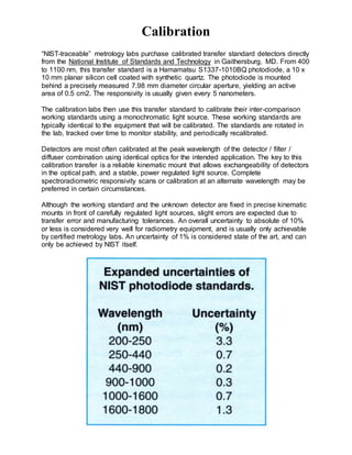
“NIST-traceable” metrology labs purchase calibrated transfer standard detectors directly
from the National Institute of Standards and Technology in Gaithersburg, MD. From 400
to 1100 nm, this transfer standard is a Hamamatsu S1337-1010BQ photodiode, a 10 x
10 mm planar silicon cell coated with synthetic quartz. The photodiode is mounted
behind a precisely measured 7.98 mm diameter circular aperture, yielding an active
area of 0.5 cm2. The responsivity is usually given every 5 nanometers.
The calibration labs then use this transfer standard to calibrate their inter-comparison
working standards using a monochromatic light source. These working standards are
typically identical to the equipment that will be calibrated. The standards are rotated in
the lab, tracked over time to monitor stability, and periodically recalibrated.
Detectors are most often calibrated at the peak wavelength of the detector / filter /
diffuser combination using identical optics for the intended application. The key to this
calibration transfer is a reliable kinematic mount that allows exchangeability of detectors
in the optical path, and a stable, power regulated light source. Complete
spectroradiometric responsivity scans or calibration at an alternate wavelength may be
preferred in certain circumstances.
Although the working standard and the unknown detector are fixed in precise kinematic
mounts in front of carefully regulated light sources, slight errors are expected due to
transfer error and manufacturing tolerances. An overall uncertainty to absolute of 10%
or less is considered very well for radiometry equipment, and is usually only achievable
by certified metrology labs. An uncertainty of 1% is considered state of the art, and can
only be achieved by NIST itself.

2. .
Choosing Input Optics
When selecting input optics for a measurement application, consider
both the size of the source and the viewing angle of the intended real-
world receiver.
Suppose, for example, that you were measuring the erythe
mal (sunburn) effect of the sun on human skin. While the sun may be
considered very much a point source, skylight, refracted and reflected
by the atmosphere, contributes significantly to the overall amount of
light reaching the earth’s surface. Sunlight is a combination of a point
source and a 2π steradian area source.
The skin, since it is relatively flat and diffuse, is an effective cosine
receiver. It absorbs radiation in proportion to the incident angle of the
light. An appropriate measurement system should also have a cosine
response. If you aimed the detector directly at the sun and tracked the
sun's path, you would be measuring the maximum irradiance. If,
however, you wanted to measure the effect on a person laying on the
beach, you might want the detector to face straight up, regardless of the
sun’s position.
Different measurement geometries necessitate specialized input optics. Radiance and
luminance measurements require a narrow viewing angle (< 4°) in order to satisfy the
conditions underlying the measurement units. Power measurements, on the other hand,
require a uniform response to radiation regardless of input angle to capture all light.
There may also be occasions when the need for additional signal or the desire to
exclude off-angle light affects the choice of input optics. A high gain lens, for example, is
often used to amplify a distant point source. A detector can be calibrated to use any
input optics as long as they reflect the overall goal of the measurement.
Cosine Diffusers
A bare silicon cell has a near perfect
cosine response, as do all diffuse
planar surfaces. As soon as you place

3. a filter in front of the detector, however, you change the spatial responsivity of the cell
by restricting off-angle light. Fused silica or optical quartz with a ground (rough) internal
hemisphere makes an excellent diffuser with adequate transmission in the ultraviolet.
Teflon is an excellent alternative for UV and visible applications, but is not an effective
diffuser for infrared light. Lastly, an integrating sphere coated with BaSO4 or PTFE
powder is the ideal cosine receiver, since the planar sphere aperture defines the cosine
relationship.
Radiance Lens Barrels
Radiance and luminance optics
frequently employ a dual lens
system that provides an
effective viewing angle of less than 4°. The tradeoff of a restricted viewing angle is a
reduction in signal. Radiance optics merely limit the viewing angle to less than the
extent of a uniform area source. For very small sources, such as a single element of an
LED display, microscopic optics are required to “underfill” the source.
The Radiance barrel shown below has a viewing angle of 3°, but due to the dual lenses,
the extent of the beam is the full diameter of the first lens; 25 mm. This provides
increased signal at close distances, where a restricted viewing angle would limit the
sampled area.
Fiber Optics
Fiber optics allow measurements in tight places or where irradiance levels and heat are
very high. Fiber optics consist of a core fiber and a jacket with an index of refraction
chosen to maximize total internal reflection. Glass fibers are suitable for use in the
visible, but quartz or fused silica is required for transmission in the ultraviolet. Fibers are
often used to continuously monitor UV curing ovens, due to the attenuation and heat
protection they provide. Typical fiber optics restrict the field of view to about ±20° in the
visible and ±10° in the ultraviolet.

4. Integrating Spheres
An integrating sphere is a hollow
sphere coated inside with Barium
Sulfate, a diffuse white reflectance
coating that offers greater than 97%
reflectance between 450 and 900 nm.
The sphere is baffled internally to
block direct and first-bounce light.
Integrating spheres are used as
sources of uniform radiance and as input optics for measuring total power. Often, a
lamp is place inside the sphere to capture light that is emitted in any direction.
High Gain Lenses
In situations with low irradiance from a point source, high gain input
optics can be used to amplify the light by as much as 50 times while
ignoring off angle ambient light. Flash sources such as tower
beacons often employ Fresnel lenses, making near field
measurements difficult. With a high gain lens, you can measure a
flash source from a distance without compromising signal strength.
High gain lenses restrict the field of view to ±8°, so cannot be used
in full immersion applications where a cosine response is required.

5. Choosing a Radiometer
Detectors translate light energy into an electrical current. Light striking a silicon
photodiode causes a charge to build up between the internal "P" and "N" layers. When
an external circuit is connected to the cell, an electrical current is produced. This current
is linear with respect to incident light over a 10 decade dynamic range.
A wide dynamic range is a prerequisite for most applications. The radiometer should be
able to cover the entire dynamic range of any detector that will be plugged into it. This
usually means that the instrument should be able to cover at least 7 decades of
dynamic range with minimal linearity errors. The current or voltage measurement device
should be the least significant source of error in the system.
Billion-to-One Dynamic Range:
Sunny Day 100,000. lux
Office Lights 1000. lux
Full Moon 0.1 lux
Overcast Night 0.0001 lux
The second thing to consider
when choosing a radiometer is
the type of features offered.
Ambient zeroing, integration
ability, and a “hold” button
should be standard. The ability
to multiplex several detectors to
a single radiometer or control
the instrument remotely may
also be desired for certain
applications. Synchronous
detection capability may be
required for low level signals. Lastly, poratbility and battery life may be an issue for
measurements made in the field.
Floating Current to Current Amplification
International Light radiometers amplify current using a floating current to-current
amplifier (FCCA), which mirrors and boosts the input current directly while “floating”
completely isolated. The FCCA current amplifier covers an extremely large dynamic
range without changing gain. This proprietary amplification technique is the key to our
unique analog to digital conversion, which would be impossible without linear current
preamplification.

6. We use continuous wave integration to integrate (or sum) the incoming
amplified current as a charge, in a capacitor. When the charge in the
capacitor reaches a threshold, a charge packet is released. This is
analogous to releasing a drop from an eye dropper. Since each drop is an
identical known volume, we can determine the total volume by counting the
total number of drops. The microprocessor simply counts the number of
charge packets that are released every 500 milliseconds. Since the clock
speed of the computer is much faster than the release of charge packets, it
can measure as many as 5 million, or as few as 1 charge packet, each 1/2
second. On the very low end, we use a rolling average to enhance the
resolution by a factor of 4, averaging over a 2 second period. The
instrument can cover 6 full decades without any physical gain change!
In order to boost the dynamic range even further, we use a single gain change of 1024
to overlap two 6 decade ranges by three decades, producing a 10 decade dynamic
range. This “range hysteresis” ensures that the user remains in the middle of one of the
working ranges without the need to change gain. In addition, the two ranges are locked
together at a single point, providing a step free transition between ranges. Even at a
high signal level, the instrument is still sensitive to the smallest charge packet, for a
resolution of 21 bits within each range! With the 10 bit gain change, we overlap two 21
bit ranges to achieve a 32 bit Analog to Digital conversion, yielding valid current
measurements from a resolution of 100 femtoamps (10-13 A) to 2.0 milliamps (10-3 A).
The linearity of the instrument over its entire dynamic range is guaranteed, since it is
dependent only on the microprocessor's ability to keep track of time and count, both of
which it does very well.
Transimpedance Amplification
Transimpedance amplification is the most common type of signal amplification,
where an op-amp and feedback resistor are employed to amplify an
instantaneous current. Transimpedance amplifiers are excellent for measuring
within a fixed decade range, but must change gain by switching feedback
resistors in order to handle higher or lower signal levels. This gain change
introduces significant errors between ranges, and precludes the instrument
from measuring continuous exposures.
A graduated cylinder is a good analogy for describing some of the limitations of
transimpedance amplification. The graduations on the side of the cylinder are the
equivalent of bit depth in an A-D converter. The more graduating lines, the greater the
resolution in the measurement. A beaker cannot measure volumes greater than itself,
and lacks the resolution for smaller measurements. You must switch to a different size
container to expand the measurement range - the equivalent of changing gain in an
amplifier.
In a simple light meter, incoming light induces a voltage, which is amplified and
converted to digital using an analog-to -digital converter. A 10 bit A-D converter
provides a total of 1024 graduations between 0 and 1 volt, allowing you to measure
between 100 and 1000 to an accuracy of 3 significant digits. To measure between 10
and 100, however, you must boost the gain bya factor of 10, because the resolution of

7. the answer is only two digits. Similarly, to measure between 1 and 10 you must boost
the gain by a factor of 100 to get three digit resolution again. In transimpedance
systems, the 100% points for each range have tobe adjusted and set to an absolute
standard. It is expected for a mismatch to occur between the 10% point of one range
and the 100% point of the range below it. Any nonlinearity or zero offset error is
magnified at this 10% point.
Additionally, since voltage is sampled instantaneously, it suffers from a lower S/N ratio
than an integrating amplifier. Transimpedance amplifiers simulate integration by taking
multiple samples and calculating the average reading. This technique is sufficient if the
sampling rate is at least double the frequency of the measured signal.
Integration
The ability to sum all of the incident light over a period of time is a very desirable
feature. Photographic film is a good example of a simple integration. The image on the
emulsion becomes more intense the longer the exposure time. An integrating
radiometer sums the irradiance it measures continuously, providing an accurate
measure of the total exposure despite possible changes in the actual irradiance level.
The primary difficulty most radiometers have with integration is range changes. Any
gain changes in the amplification circuitry mean a potential loss of data. For applications
with relatively constant irradiance, this is not a concern. In flash integration, however,
the change in irradiance is dramatic and requires specialized amplification circuitry for
an accurate reading.
Flash integration is preferable to measuring the peak irradiance, because the duration
of a flash is as important as its peak. In addition, since the total power from a flash is
low, an integration of 10 flashes or more will significantly improve the signal to noise
ratio and give an accurate average flash. Since International Light radiometers can
cover a large dynamic range (6 decades or more) without changing gain, the
instruments can accurately subtract a continuous low level ambient signal while
catching an instantaneous flash without saturating the detector.
The greatest benefit of integration is that it cancels out noise. Both the signal and the
noise vary at any instant in time, although they are presumably constant in the average.
International Light radiometers integrate even in signal mode, averaging over a 0.5
second sampling period to provide a significant improvement in signal to noise ratio.
Zero
The ability to subtract ambient light and noise from readings is a necessary feature for
any radiometer. Even in the darkest room, electrical “dark current” in the photodiode
must be subtracted. Most radiometers offer a “Zero” button that samples the ambient
scatter and electrical noise, subtracting it from subsequent readings.
Integrated readings require ambient subtraction as well. In flash measurements
especially, the total power of the DC ambient could be higher than the power from an
actual flash. An integrated zero helps to overcome this signal to noise dilemma

8. Choosing a Filter
Spectral Matching
A detector’s overall spectral sensitivity is equal to the product of the
responsivity of the sensor and the transmission of the filter. Given a desired
overall sensitivity and a known detector responsivity, you can then solve for the
ideal filter transmission curve.
A filter’s bandwidth decreases with thickness, in accordance with Bouger’s law
(see Chapter 3). So by varying filter thickness, you can selectively modify the
spectral responsivity of a sensor to match a particular function. Multiple filters
cemented in layers give a net transmission equal to the product of the individual
transmissions. At International Light, we’ve written simple algorithms to
iteratively adjust layer thicknesses of known glass melts and minimize the error
to a desired curve.
Filters operate by absorption or interference. Colored glass filters are doped
with materials that selectively absorb light by wavelength, and obey Bouger’s
law. The peak transmission is inherent to the additives, while bandwidth is
dependent on thickness. Sharp-cut filters act as long pass filters, and are often
used to subtract out long wavelength radiation in a secondary measurement.
Interference filters rely on thin layers of dielectric to cause interference between
wavefronts, providing very narrow bandwidths. Any of these filter types can be
combined to form a composite filter that matches a particular photochemical or
photobiological process.

12. Choosing a Detector
Sensitivity
Sensitivity to the band of interest is a primary consideration when choosing a detector.
You can control the peak responsivity and bandwidth through the use of filters, but you
must have adequate signal to start with. Filters can suppress out of band light but
cannot boost signal.
Another consideration is blindness to out of band radiation. If you are measuring solar
ultraviolet in the presence of massive amounts of visible and infrared light, for example,
you would select a detector that is insensitive to the long wavelength light that you
intend to filter out.
Lastly, linearity, stability and durability are considerations. Some detector types must be
cooled or modulated to remain stable. required for other types. In addition, some can be
burned out by excessive light, or have their windows permanently ruined by a
fingerprint.
Silicon Photodiodes
Planar diffusion type silicon photodiodes are perhaps the
most versatile and reliable sensors available. The P-layer
material at the light sensitive surface and the N material
at the substrate form a P-N junction which operates as a
photoelectric converter, generating a current that is
proportional to the incident light. Silicon cells operate
linearly over a ten decade dynamic range, and remain
true to their original calibration longer than any other type
of sensor. For this reason, they are used as transfer

13. standards at NIST.
Silicon photodiodes are best used in the short-circuit mode, with zero input impedance
into an op-amp. The sensitivity of a light-sensitive circuit is limited by dark current, shot
noise, and Johnson (thermal) noise. The practical limit of sensitivity occurs for an
irradiance that produces a photocurrent equal to the dark current (Noise Equivalent
Power, NEP = 1).
Solar-Blind Vacuum Photodiodes
The phototube is a light sensor that is based on the
photoemissive effect.
The phototube is a bipolar tube which consists of a
photoemissive cathode surface that emits electrons in
proportion to incident light, and an anode which collects the
emitted electrons. The anode must be biased at a high voltage
(50 to 90 V) in order to attract electrons to jump through the
vacuum of the tube. Some phototubes use a forward bias of
less than 15 volts, however.
The cathode material determines the spectral
sensitivity of the tube. Solar-blind vacuum
photodiodes use Cs-Te cathodes to provide
sensitivity only to ultraviolet light, providing as
much as a million to one long wavelength
rejection. A UV glass window is required for
sensitivity in the UV down to 185 nm, with
fused silica windows offering transmission
down to 160 nm.

14. Multi-Junction Thermopiles
The thermopile is a heat sensitive device that measures
radiated heat.
The sensor is usually sealed in a vacuum to prevent heat
transfer except by radiation. A thermopile consists of a
number of thermocouple junctions in series which convert
energy into a voltage using the Peltier effect. Thermopiles
are convenient sensor for measuring the infrared, because
they offer adequate sensitivity and a flat spectral response in
a small package. More sophisticated bolometers and pyroelectric detectors need to be
chopped and are generally used only in calibration labs.
Thermopiles suffer from temperature drift, since the reference portion of the detector is
constantly absorbing heat. The best method of operating a thermal detector is by
chopping incident radiation, so that drift is zeroed out by the modulated reading.
The quartz window in most thermopiles is adequate for transmitting from 200 to 4200
nm, but for long wavelength sensitivity out to 40 microns, Potassium Bromide windows
are used.

15. Graphing Data
Line Sources
Discharge sources emit large amounts of irradiance at particular atomic spectral lines,
in addition to a constant, thermal based continuum. The most accurate way to portray
both of these aspects on the same graph is with a dual axis plot, shown in figure 9.1.
The spectral lines are graphed on an irradiance axis (W/cm2) and the continuum is
graphed on a band irradiance (W/cm2/nm) axis. The spectral lines ride on top of the
continuum.
Another useful way to graph mixed sources is to plot spectral lines as a rectangle the
width of the monochromator bandwidth. (see fig. 5.6) This provides a good visual
indication of the relative amount of power contributed by the spectral lines in relation to
the continuum, with the power being bandwidth times magnitude.
The best way to represent the responsivity of a detector with respect to incident angle of
light is by graphing it in Polar Coordinates. The polar plot in figure 9.2 shows three
curves: A power response (such as a laser beam underfilling a detector), a cosine
response (irradiance overfilling a detector), and a high gain response (the effect of using
a telescopic lens). This method of graphing is desirable, because it is easy to
understand visually. Angles are portrayed as angles, and responsivity is portrayed
radially in linear graduations.

16. The power response curve clearly shows that the response between -60 and +60
degrees is uniform at 100 percent. This would be desirable if you were measuring a
laser or focused beam of light, and underfilling a detector. The uniform response means
that the detector will ignore angular misalignment.
The cosine response is shown as a circle on the graph. An irradiance detector with a
cosine spatial response will read 100 percent at 0 degrees (straight on), 70.7 percent at
45 degrees, and 50 percent at 60 degrees incident angle. (Note that the cosines of 0°,
45° and 60°, are 1.0, 0.707, and 0.5, respectively).
The radiance response curve has a restricted field of view of ± 5°. Many radiance
barrels restrict the field of view even further (± 1-2° is common). High gain lenses
restrict the field of view in a similar fashion, providing additional gain at the expense of
lost off angle measurement capability.
The Cartesian graph in figure 9.3 contains the same data as the polar plot in figure 9.2
on the previous page. The power and high gain curves are fairly easy to interpret, but
the cosine curve is more difficult to visually recognize. Many companies give their
detector spatial responses in this format, because it masks errors in the cosine
correction of the diffuser optics. In a polar plot the error is easier to recognize, since the
ideal cosine response is a perfect circle.
In full immersion applications such as phototherapy, where light is coming from all
directions, a cosine spatial response is very important. The skin (as well as most
diffuse, planar surfaces) has a cosine response. If a cosine response is important to
your application, request spatial response data in polar format.

17. At the very least, the true cosine response should be superimposed over the Cartesian
plot of spatial response to provide some measure of comparison.
Note: Most graphing software packages do not provide for the creation of polar axes.
Microsoft Excel™, for example, does have “radar” category charts, but does not support
polar scatter plots yet. SigmaPlot™, an excellent scientific graphing package, supports
polar plots, as well as custom axes such as log-log etc. Their web site is:
http://www.spss.com/
A log plot portrays each 10 to 1 change as a fixed linear displacement. Logarithmically
scaled plots are extremely useful at showing two important aspects of a data set. First,
the log plot expands the resolution of the data at the lower end of the scale to portray
data that would be difficult to see on a linear plot. The log scale never reaches zero, so
data points that are 1 millionth of the peak still receive equal treatment. On a linear plot,
points near zero simply disappear.
The second advantage of the log plot is that percentage difference is represented by the
same linear displacement everywhere on the graph. On a linear plot, 0.09 is much
closer to 0.10 than 9 is to 10, although both sets of numbers differ by exactly 10
percent. On a log plot, 0.09 and 0.10 are the same distance apart as 9 and 10, 900 and
1000, and even 90 billion and 100 billion. This makes it much easier to determine a
spectral match on a log plot than a linear plot.

18. As you can clearly see in figure 9.4, response B is within 10 percent of response A
between 350 and 400 nm. Below 350 nm, however, they clearly mismatch. In fact, at
315 nm, response B is 10 times higher than response
A. This mismatch is not evident in the linear plot, figure 9.5, which is plotted with the
same data.
One drawback of the log plot is that it compresses the data at the top end, giving the
appearance that the bandwidth is wider than it actually is. Note that Figure 9.4 appears
to approximate the UVA band.
Most people are familiar with graphs that utilize linearly scaled axes. This type of graph
is excellent at showing bandwidth, which is usually judged at the 50 percent power
points. In figure 9.5, it is easy to see that response A has a bandwidth of about 58 nm
(332 to 390 nm). It is readily apparent from this graph that neither response A nor
response B would adequately cover the entire UVA band (315 to 400 nm), based on the
location of the 50 percent power points. In the log plot of the same data (fig. 9.4), both
curves appear to fit nicely within the UVA band.

19. This type of graph is poor at showing the effectiveness of a spectral match across an
entire function. The two responses in the linear plot appear to match fairly well. Many
companies, in an attempt to portray their products favorably, graph detector responses
on a linear plot in order to make it seem as if their detector matches a particular photo-
biological action spectrum, such as the Erythemal or Actinic functions. As you can
clearly see in the logarithmic curve (fig. 9.4), response A matches response B fairly well
above 350 nm, but is a gross mismatch below that. Both graphs were created from the
same set of data, but convey a much different impression.
As a rule of thumb - half power bandwidth comparisons and peak spectral response
should be presented on a linear plot. Spectral matching should be evaluated on a log
plot.
The Diabatie scale (see fig. 9.7) is a log-log scale used by filter glass manufacturers to
show internal transmission for any thickness. The Diabatie value, θ(λ), is defined as
follows according to DIN 1349:
θ(λ) = 1 - log(log(1/τ))
Linear transmission curves are only useful for a single thickness (fig. 9.6). Diabatie
curves retain the same shape for every filter glass thickness, permitting the use of a
transparent sliding scale axis overlay, usually provided by the glass manufacturer. You
merely line up the key on the desired thickness and the transmission curve is valid.

21. Setting Up an Optical Bench
A Baffled Light Track
The best light measurement setup controls as many variables as possible. The idea is
to prevent the measurement environment from influencing the measurement.
Otherwise, the measurement will not be repeatable at a different time and place.
Baffles, for example, greatly reduce the influence of stray light reflections. A baffle is
simply a sharp edged hole in a piece of thin sheet metal that has been painted black.
Light outside of the optical beam is blocked and absorbed without affecting the optic
Multiple baffles are usually required in order to guarantee that light is trapped once it
strikes a baffle. The best light trap of all, however, is empty space. It is a good idea to
leave as much space between the optical path and walls or ceilings as is practical. Far
away objects make weak reflective sources because of the Inverse Square Law.
Objects that are near to the detector, however, have a significant effect, and should be
painted with “black velvet” paint or moved out of view.
A shutter, door, or light trap in one of the baffles allows you to measure the background
scatter component and subtract it from future readings. The “zero” reading should be
made with the source ON, to maintain the operating temperature of the lamp as well as
measure light that has defeated your baffling scheme.

22. Kinematic Mounts
Accurate distance
measurements and
repeatable positioning in
the optical path are the
most important
considerations when
setting up an otical bench.
The goal of an optical
bench is to provide
repeatability. It is not
enough to merely control
the distance to the source,
since many sources have
non-uniform beams. A
proper detector mounting
system provides for
adjustment of position and
angle in 3-D space, as well
as interchangeability into a
calibrated position in the optical path.
To make a kinematic fixture, cut a cone and a conical slot into a piece of metal using a
45° conical end mill (see fig. 8.2). A kinematic mount is a three point fixture, with the
third point being any planar face. The three mounting points can be large bolts that have
been machined into a ball on one end, or commercially available 1/4-80 screws with ball
bearing tips (from Thorlabs, Inc.) for small fixtures.
The first leg rests in the cone hole, fixing the position of that leg as an X-Y point. The
ball tip ensures that it makes reliable, repeatable contact with the cone surface. The
second leg sits in the conical slot, fixed only in Yaw, or angle in the horizontal plane.
The use of a slot prevents the Yaw leg from competing with the X-Y leg for control. The
third leg rests on any flat horizontal surface, fixing the Pitch, or forward tilt, of the
assembly.
A three legged detector carrier sitting on a kinematic mounting plate is the most
accurate way to interchange detectors into the optical path, allowing intercomparisons
between two or more detectors.
Bibliography
http://www.intl-lighttech.com/support/light-measurement-calibration-chapter-14-light-measurement-
tutorial

23. RIZAL TECHNOLOGICAL UNIVERSITY
BONI MANDALUYONG
COLLEGE OF ENGINEERING AND INDUSTRIAL TECHNOLOGY
BACHELOR OF SCIENCE IN ELECTRICAL ENGINEERING
(Illuminationg Engineering Design)
Aljon Garcia
Kevin Dimaandal
Melaiza Jean Lacson
Dandrift Figueroa
John Royces Valencia
Isaac Delos santos
Arjenly Valiente
Engr. Arnold Ilagas
September 6, 2015