Automated detection of driver fatigue based on EEG signals using gradient boosting decision tree model.pdf

BRIEF COMMUNICATION
Automated detection of driver fatigue based on EEG signals using
gradient boosting decision tree model
Jianfeng Hu1 • Jianliang Min1
Received: 21 October 2017 / Revised: 13 March 2018 / Accepted: 11 April 2018
Ó Springer Science+Business Media B.V., part of Springer Nature 2018
Abstract
Driver fatigue is increasingly a contributing factor for traffic accidents, so an effective method to automatically detect
driver fatigue is urgently needed. In this study, in order to catch the main characteristics of the EEG signals, four types of
entropies (based on the EEG signal of a single channel) were calculated as the feature sets, including sample entropy, fuzzy
entropy, approximate entropy and spectral entropy. All feature sets were used as the input of a gradient boosting decision
tree (GBDT), a fast and highly accurate boosting ensemble method. The output of GBDT determined whether a driver was
in a fatigue state or not based on their EEG signals. Three state-of-the-art classifiers, k-nearest neighbor, support vector
machine and neural network were also employed. To assess our method, several experiments including parameter setting
and classification performance comparison were performed on 22 subjects. The results indicated that it is possible to use
only one EEG channel to detect a driver fatigue state. The average highest recognition rate in this work was up to 94.0%,
which could meet the needs of daily applications. Our GBDT-based method may assist in the detection of driver fatigue.
Keywords Driver fatigue Electroencephalogram (EEG) Gradient boosted decision tree (GBDT) Entropy
Introduction
A worldwide increase in traffic accidents have resulted in
very large casualties with driver fatigue named as one of
the most important causes. Driver fatigue is the transitory
period between wakefulness and sleep, which can lead to
sleep if not interrupted. Driver fatigue has been defined as a
state that reduces psychological alertness, which can affect
performance in cognitive and psychomotor tasks such as
driving. The automatic detection of driver fatigue is a
meaningful research field in the driving safety assistance
system (Lal and Craig 2001; Saini and Saini 2014). Many
methods have been proposed in the past few years,
including various vehicle sensor parameters (Sahayadhas
et al. 2012), eye state (Lin et al. 2015), video imaging
techniques (Jo et al. 2014), and physiological signals.
Furthermore, some methods have been specially developed
to detect driver fatigue via using electromyograms (EMG)
(Wang 2015; Fu and Wang 2014), electrocardiograms
(ECG) (Fu and Wang 2014), electrooculograms (EOG)
(Ma et al. 2014), and electroencephalograms (EEG) (Cor-
rea et al. 2014; Mu et al. 2017; Yin et al. 2017; Wang et al.
2018), where EEG is considered the most common and
effective way to identify driver fatigue as the direct reac-
tion of the brain states (Kar et al. 2010). Furthermore, EEG
has been widely used in various fields nowadays, especially
computer signal recognition (Dietrich and Kanso 2010;
Donoghue et al. 2015; Shalbaf et al. 2015; Swapna et al.
2013; Mumtaz et al. 2017).
Various approaches based on EEG signals have been
developed to detect driver fatigue. Chai et al. (2016) pre-
sented an autoregressive (AR) model for feature extraction
and a Bayesian neural network for the classification algo-
rithm, where they achieved a highest accuracy of 88.2%.
Nguyen et al. (2017) proposed a new approach for com-
bining EEG, EOG, ECG and NIRS signals to detect driver
drowsiness based on fisher’s linear discriminant analysis
method and achieved the mean result with 79.2 (± 9.4) of
9 subjects. Li et al. (2012) collected 16 channels of EEG
data and computed 12 types of energy parameters, and
Jianfeng Hu
huguess211@hotmail.com
1
The Center of Collaboration and Innovation, Jiangxi
University of Technology, Ziyang Road,
Nanchang 330098, Jiangxi Province, China
123
Cognitive Neurodynamics
https://doi.org/10.1007/s11571-018-9485-1(0123456789().,-volV)
(0123456789().,-volV)

obtained the highest accuracy of 91.5% from two channels
(FP1 and O1). Chai et al. (2017) presented an improvement
of classification performance for EEG-based driver fatigue
classification from 43 participants by using AR feature
extractor and sparse-deep belief networks, obtained an
improved classification performance with a sensitivity of
93.9%, a specificity of 92.3%, an accuracy of 93.1%.
Xiong et al. (2016) combined features of AE and SE with
an SVM classifier and achieved the highest accuracy of
91.3% at channel P3. Fu et al. (2016) proposed a fatigue
detection model based on the Hidden Markov Model
(HMM), and achieved the highest accuracy of 92.5% based
on EEG signals of two channels (O1 and O2) and other
physiological signals. Silveira et al. (2016) proposed a
method for assessing alertness level based on a single EEG
channel (Pz–Oz) by using the normalized Haar discrete
wavelet packet transform, found that the second index
(c ? b)/(d ? a) achieved the best results. Shen et al.
(2007) used random forest (RF) with a heuristic initial
feature ranking scheme based on EEG signals from 12
subjects, which yielded the highest accuracy of 87.7%.
With respect to driver fatigue detection based on EEG
signals, the performance of many linear and non-linear
single classifiers has already been assessed; however, it
may be difficult to build a better single classifier as EEG
signals are unstable and the training set is usually com-
paratively small. Consequently, such classifiers may have a
poor performance or be unstable. Recent studies have
shown that ensemble classifiers perform better than single
classifiers (Hassan and Subasi 2016; Yang et al. 2016);
however, few studies have been conducted on using
ensemble classifiers based on EEG signals to study driver
fatigue detection. Nevertheless, multichannel EEG acqui-
sition systems such as the 32-channel EEG system used in
this study, can only be used in the laboratory. Therefore, an
EEG system with less channels, or even one channel,
would be more convenient, and more comfortable.
In this study, a complete study of an EEG-based driver
fatigue detection system was provided by using GBDT
including data acquisition, data processing, feature
extraction and classification. The study focused on apply-
ing a machine learning method to detect driver fatigue. The
rest of this article was organized as follows. In ‘‘Methods’’
section, the gradient boosting decision tree algorithm was
described in detail, and feature extraction was presented,
including SE, FE, AE and PE. ‘‘Results’’ section showed
that the experiments conducted on 22 subjects based on the
GBDT method, and was followed by our conclusions in
‘‘Discussion’’ section.
Methods
Subjects
Twenty-two students (8 female, 17–24 years) participated
in this experiment. All subjects had a driver’s license and
were asked to abstain from alcohol, medications, or tea
before and during the experiment. Prior to the experiment,
they practiced the driving task for several minutes to
become acquainted with the experimental procedures and
purposes. This work was approved by the Academic Ethics
Committee of Jiangxi University of Technology. The
subjects provided their written informed consent as per
human research protocol in this study.
Experimental paradigm
A sustained-attention driving task was performed by each
subject on a static driving simulator (The ZY-31D car
driving simulator, produced by Peking ZhongYu Co., Ltd).
This equipment is an analog form of a real driving car, and
contains all the driving capabilities of a vehicle. Using
computer software technology, different driving environ-
ments and conditions can be constructed, such as sunny,
foggy, or snowy weather and mountainous, highways, or
the countryside. The driving environment selected for this
experiment was a highway with low traffic density to more
easily induce monotonous driving. Some researches had
pointed out that our brains (under this type of driving
environment) were more easily turned into a fatigue state
and the EEG signals were more stable, which was good for
recording data. All subjects in this experiment had
approximate real driving experience.
Data recording and preprocessing
In summary, the total duration of the experiment was
40–120 min. The first step was to become familiar with the
simulation software, then there was continuous mono-
tonous driving until driver fatigue was determined, and the
experiment was terminated.
When the driving lasted 10 min, the last 5 min of EEG
signals were recorded as a normal state. When the con-
tinuous driving lasted between 30 and 120 min until self-
reported fatigue, the questionnaire results showed that the
subject was in driving fatigue (obeying the Chalder fatigue
scale and Lee’s subjective fatigue scale) (Lee et al. 1991;
Borg 1990) so the last 5 min of the EEG signals were
labeled as the fatigue state. EOG was also used to analyze
eye blink patterns as an objective validation of the fatigue
state. It should be noted that the validation of the fatigue
condition has also been conducted with a self-reported
123

fatigue questionnaire as per the Chalder fatigue scale and
Lee’s subjective fatigue scale in our recent researches (Mu
et al. 2017; Yin et al. 2017), and the method of using a
questionnaire for identifying fatigue condition has been
used in many other studies (Li et al. 2012; Craig et al.
2012; Liu et al. 2010). The drivers were required to com-
plete all tasks and ensure safe driving. Prior to the exper-
iment, the drivers familiarized themselves with the
operation of the driving simulator and the completion of
the driving tasks.
All channel data were referenced to two electrically
linked mastoids at A1 and A2, digitized at 1000 Hz from a
32-channel electrode cap (including 30 effective channels
and two reference channels) based on the international
10–20 system and stored in a computer for offline analysis.
Eye movements and blinks were monitored by recording
the horizontal and vertical EOG.
After collecting EEG signals, the main steps of data
preprocessing were carried out by the Scan 4.3 software of
Neuroscan (Neuroscan, Compumedics, Australia). First,
the raw signals were filtered by a 0.15–45 Hz band-pass
filter to remove the noise. Next, 5 min of EEG data from
thirty electrodes were sectioned into 1-s epoch, resulting in
approximately 300 epochs. With 22 subjects, a total of
6600 units of datasets were formed for the normal state and
another 6600 units for the fatigue state. A 10-fold cross
validation approach for measuring classification results
was used.
Feature extraction
As nonlinear parameters can quantify the complexity of a
time series, it can be used to evaluate the non-linear,
unstable EEG signals (Azarnoosh et al. 2011; Mateos et al.
2017). Spectral entropy (PE) was calculated by applying
the Shannon function to the normalized power spectrum,
which was described in detail in the literature (Kannathal
et al. 2005). Approximate entropy (AE) was calculated as
proposed by Pincus (1991). Like AE, sample entropy (SE)
was calculated as proposed by Richman and Moorman
(Richman and Moorman 2000). The calculation algorithm
of AE and SE were defined clearly in the literature (Song
et al. 2012), as was fuzzy entropy (FE) (Xiang et al. 2015).
In the four above-mentioned types of entropies, AE, SE
and FE have parameters setting, m and r, which are the
dimensions of phase space and similarity tolerance,
respectively. Generally, too large an r will lead to a loss of
useful information; however, if r is under estimated, the
sensitivity to noise will increase significantly. In the pre-
sent study, m = 2 while r = 0.2 * SD, where SD denotes
the standard deviation of the time series, as refer the lit-
erature (Yentes et al. 2013).
For optimizing the detection quality, the feature sets
were normalized for each subject and each channel by
scaling between 0 and 1.
Classification
Since there is no uniform classification method suitable for
all subjects and all applications, it is useful to test ensemble
classification methods.
To assess the GBDT method for driver fatigue detection,
three widely used classifiers (KNN, SVM and NN) were
employed as a comparison. KNN is a supervised learning
technique where a new instance is classified based on the
closest training samples present in the feature space. KNN
implements learning based on the k-nearest neighbors of
each query point, where k is 10 in this study, if not
otherwise specified. In the case of nonlinear classification,
kernels (such as radial basis functions (RBF)) are used to
map the data into a higher dimensional feature space where
a linear separating hyper-plane could be found. When
training an SVM classifier with the RBF kernel (Mu et al.
2016), two parameters must be considered: c and c. A
lower c makes the decision surface smooth, while a higher
c aims at classifying all training examples correctly. c
defines how much influence a single training example has.
In this study, c = 2, and c = 1. NN is trained via using
gradient descent and the gradients calculated by using
Backpropagation (BP).
In this work, a recently developed ensemble method
named GBDT, originally derived by Friedman (Friedman
2001; Hastie et al. 2009), and was introduced into driver
fatigue detection. The GBDT-based method is based on a
greedy strategy (called gradient boosting), which is dif-
ferent from random forest which is based on bootstrap
aggregating (Bauer and Kohavi 1999). A parameter regu-
larization process can prevent such over-fitting and
improve prediction accuracy by optimizing four parame-
ters: number of boosting stages (N), learning rate (L),
maximum depth (M), and fraction of samples (F).
Performance metrics
To estimate the potential application performance of a
detector, it is very important to properly examine the
detection quality. The total average accuracy based on a
feature set and some classifiers was the average of the
accuracy of all single channel based on the same feature
and the same classifier. The classification capabilities of
different classifiers were comprehensively investigated
with several indexes including Accuracy, Precision, Recall,
F1-score, Matthews Correlation Coefficient (MCC), and
the Brier score (Sokolova et al. 2006). These indexes are
given as follows: Accuracy is the percentage of normal
123

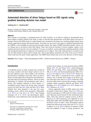
predictions corresponding to all samples; Precision is the
percentage of normal predictions corresponding to the
normal samples; and Recall is the percentage of fatigue
predictions corresponding to the fatigue samples. Further-
more, F1-score was used to appraise both Precision and
Recall. The MCC was used as a measure of the quality of
binary classifications as it considers true and false positives
and negatives, and is generally regarded as a balanced
measure which can be used even if the classes are of very
different sizes. The Brier score measures the mean squared
difference between the predicted probability assigned to
the possible outputs and the actual output. Therefore, a
lower Brier score value and higher Precision, Recall, F1-
score, and MCC values relates to higher performance.
Receiver Operating Characteristic (ROC) analysis is a
kind of reliability estimation, and ROC curves regard each
detection result as the possible critical value of diagnosis.
The area under the ROC curve (AUC) is accepted as a fair
indicator of measuring classifier performance since it is
invariant to the operating conditions such as different
misclassification costs and skewed class distribution
(Bradley 1997).
Results
To validate the model performance of different combina-
tions of regularization parameters, a series of GBDT
models were built with various boosting stages
(N = 50–2000), learning rate (L = 1.0–0.001), maximum
depth (M = 1–7), and fraction of samples (F = 0.5–1.0).
For the four feature sets, the performances of GBDT
Fig. 1 Performance of different
classifiers and the GBDT
method with different number
of boosting stages. The left
vertical coordinate is for
average accuracy, while the
horizontal coordinate is for
classifier: KNN, SVM, NN,
GBDT (with N = 50), GBDT
(with N = 100), GBDT (with
N = 200), GBDT (with
N = 500), GBDT (with
N = 1000) and GBDT (with
N = 2000), respectively. Where
L = 0.1, M = 3, F = 1. GB50,
GB100, GB200, GB500,
GB1000 and GB2000 represent
the GBDT ensemble classifier
with 50, 100, 200, 500, 1000
and 2000 boosting stages,
respectively
123

models based on different combination of regularization
parameters are described in the following figures.
To examine the effectiveness of the GBDT model used
for driver fatigue detection, a comparison was conducted
with other commonly used classifiers including KNN,
SVM, and NN under the same conditions (using the same
data and feature sets). Figure 1 shows a comparison
between the results for the four feature sets, respectively. In
this study, Accuracy, Precision, Recall, F1-score, MCC,
and the Brier score were used as the model performance
indicators. A comparison of the results of different pre-
diction methods and feature sets indicated that the GBDT
model was statistically different to any of other techniques,
and received the best model performance out of all four
feature sets. This finding further confirmed the advantages
of the GBDT model in modeling complex relationships
between EEG signals and the fatigue state.
As shown in Fig. 1, the feature set FE outperformed the
other three feature sets in all views of the six indexes. The
average accuracy using feature set FE achieved 0.919
(when N = 500), which was more than seven percentage
points off set PE (accuracy = 0.848).
The influence of the number of boosting stages (N) on
model performance can also be seen in Fig. 1. Given other
parameters, as N increased, the model obtained a better
performance; however, when the value of the shrinkage
parameter reached a certain level, the model performance
reached equilibrium. Taking feature set FE as an example,
the model performance became better (accuracy increasing
from 0.850–0.919) as the learning rate parameter value
increased from N = 50 to N = 500. However, increasing
the value of the learning rate parameter from N = 500 to
N = 2000 led to few changes (paired t test, p [ 0.05).
The highest average accuracy of a single channel
reached 0.920, which was very competitive compared to
research described in Introduction. Even for the weak
feature set (such as feature set PE), GBDT could signifi-
cantly improve the performance from 0.541 (using
Fig. 2 Performance of GBDT
method with different learning
rates. The left vertical
coordinate is for Accuracy,
while the horizontal coordinate
is for classifier: GBDT (with
L = 0.001), GBDT (with
L = 0.1), GBDT (with L = 0.5)
and GBDT (with L = 1),
respectively. LR0001, LR0005,
LR001, LR005, LR01, LR05
and LR1 represent the GBDT
ensemble classifier with
learning rates of 0.001, 0.005,
0.01, 0.05, 0.1, 0.5 and 1.0,
respectively. Where N = 500,
M = 3, F = 1
123

classifier NN) to 0.851 (GBDT1000). Thus, it appears that
GBDT could reduce the difference between the different
feature sets, for example, the difference in average accu-
racy between feature set FE and feature set PE based on
classifier SVM was 0.247 while the difference in average
accuracy between feature set FE and feature set PE based
on GBDT was 0.069. This may result from the GBDT
model being able to effectively enhance the effect of the
weaker feature sets.
The parameter learning rate strongly interacted with the
number of boosting stages. Hastie recommended that the
learning rate was set to a small constant (e.g., learning
rate = 0.1) (Hastie et al. 2009). The influence of the
learning rate parameter on model performance can be seen
in Fig. 2. Given the boosting stage (N = 500), an increased
value of the learning rate parameter required fewer trees
and less computational time to achieve its minimum error.
Taking feature set FE as an example, the model perfor-
mance became better (accuracy increased from 0.816 to
0.908) as the learning rate increased from L = 0.001 to
L = 0.1. However, increasing the value of the learning rate
parameter from L = 0.1 to L = 1 led to an insignificant
result (paired t test, p [ 0.05).
Even for the weak feature set, such as feature set PE,
GBDT could significantly improve the performance from
0.582 (LR0001) to 0.851 (LR05). The difference in average
on LR0001 was 0.234, while the difference in average
on LR05 was 0.069.
The influence of the maximum depth on model perfor-
mance can be seen in Fig. 3. For a given boosting stage
Fig. 3 Performance of the
GBDT method with different
maximum depths. The left
horizontal coordinate is the
classifier: GBDT (with M = 1),
GBDT (with M = 2), GBDT
(with M = 3), GBDT (with
M = 4), GBDT (with M = 5),
GBDT (with M = 6) and GBDT
(with M = 7), respectively.
Md1, Md2, Md3, Md4, Md5,
Md6 and Md7 represent the
GBDT ensemble classifier with
maximum depths of 1, 2, 3, 4, 5,
6 and 7, respectively. Where
L = 0.1, N = 500, F = 1
123

(N = 500) and learning rate (L = 0.1), as maximum depth
changed, the model obtained different performances. Tak-
ing feature set FE as an example, the model performance
became better (accuracy increased from 0.814 to 0.920) as
the learning rate parameter value increased from M = 1 to
M = 3. However, an increase in the value of maximum
depth from M = 3 to M = 7 led to no significant changes
(paired t test, p [ 0.05). Even for the weak feature set, such
Fig. 4 Performance of the
GBDT method with a different
fraction of samples. The left
horizontal coordinate is the
classifier: GBDT (with F = 0.5),
GBDT (with F = 0.6), GBDT
(with F = 0.7), GBDT (with
F = 0.8), GBDT (with
F = 0.85), GBDT (with F = 0.9)
and GBDT (with F = 1),
respectively. Sub05, Sub06,
Sub07, Sub08, Sub085, Sub09
and Sub1 represent the GBDT
ensemble classifier with the
fraction of samples being 0.5,
0.6, 0.7, 0.8, 0.85, 0.9 and 1.0,
respectively, where L = 0.1,
M = 3, N = 500
Fig. 5 ROC Curve
Table 1 The paired-samples t test analysis between different
classifiers
KNN SVM NN GB50 GB200 GB500 GB1000
SVM *
NN * **
GB100 ** * **
GB200 ** ** ** **
GB500 q * ** ** *
GB1000 * q q q * q
GB2000 q q * ** q q q
*p 0.05; **p 0.01; qp [ 0.05
123

as feature set PE, GBDT could significantly improve per-
formance from 0.826 (md1) to 0.919 (md3). The difference
in average accuracy between feature set FE and feature set
PE based on Md1 was 0.16, while the difference in average
on md3 was 0.068.
The influence of fraction of samples on model perfor-
mance can be seen in Fig. 4. For a given boosting stage
(N = 500) and learning rate (L = 0.1), as fraction of sam-
ples increased, the model obtained a better performance.
Taking feature set FE as an example, the model perfor-
mance became better (accuracy increased from 0.588 to
0.920) as the fraction of samples increased from F = 0.5 to
F = 1. Even for the weak feature set, such as feature set PE,
GBDT could significantly improve performance from
0.549 (Sub05) to 0.851 (Sub1). Unlike the preceding
example, the difference in average accuracy between fea-
ture set FE and feature set PE based on Sub05 was 0.038,
while the difference in average accuracy between feature
set FE and feature set PE based on Sub1 was 0.069.
The highest accuracy of a single channel reached 0.940
based on a combination of channel TP7 and feature set FE,
or a combination of channel C4 and feature set AE. The
highest average accuracy of a single channel reached 0.919
based on feature set FE.
The ROC curve is a plot of true positive rate on the Y
axis and false positive rate on the X-axis by varying dif-
ferent threshold ratios. A random performance of a clas-
sifier would have a straight line connecting (0, 0) to (1, 1).
A ROC curve of the classifier appearing in the upper left
triangle suggest that it has a superior performance classi-
fication. The results of ten independently rounds were used
to draw mean ROC curves. The performance was analyzed
by ROC curves and areas under ROC curves (AUC). Fig-
ure 5 shows the ROC curve for all subjects based on
optimal GBDT classifiers, and the corresponding AUC was
0.946.
Discussion
In this paper, a GBDT-based approach was proposed to
detect driver fatigue in an EEG-based system. Results
showed that it is a promising system to detect driver fati-
gue, and achieved a higher success rate with only one
channel. With the purpose of providing a more efficient
ensemble method for detecting driver fatigue, it was found
that: (1) it was possible to use only one electrode for driver
fatigue detection, where the highest recognition rate of one
electrode could be up to 0.940, which was able to meet the
needs of daily applications; and (2) the GBDT method
could obviously improve the performance of the detector,
especially for the weaker feature sets. This is different from
the traditional computational intelligence algorithms (e.g.,
KNN, SVM, and NN).
But are there significant differences among them? A
paired-samples t test was conducted to compare the per-
formance using different classifiers and results show in
Table 1. By using the paired-samples t test (with double
tail), we can statistically conclude whether the factor has
significantly improved the average accuracy or not. It can
be seen that there is a significant difference between the
majorities of classifiers (p 0.05). Performance of classi-
fier GB200 and GB500 are significantly better than that of
other classifiers, while performance of classifier GB2000
significantly worse than that of other classifiers, as also
shown in Fig. 1.
Furthermore, as seen in Table 2, it was found that the
classification performance of the proposed method was
better than that in previous research using different clas-
sification methods based on fewer channels EEG signals.
Although the present study is based on the existing EEG
data, the high performance of detecting driving fatigue by
using a GBDT-based classification indicated that it can be
applied well in the real-time detection of driving fatigue.
As different brain characteristics probably exists
between different subjects, the EEG features may be
Table 2 Studies regarding driver fatigue detection using different methods
Research group Feature method Classifiers EEG channels Average accuracy
(%)
Xiong et al. (2016) AE and SE SVM P3 90.0
Correa et al. (2014) Multimodal Analysis NN C3-O1, C4-A1 and O2-
A1
83.6
Nguyen et al. (2017) Statistical tests Fisher’s linear discriminant
analysis
All channels 88.6
Ko et al. (2015) Fast Fourier
Transformation
The linear regression A single frontal channel 90.0
Chai (Chai et al. 2017) AR Sparse-DBN All channels 93.1
This paper FE GBDT TP7 94.0
123

different for different subjects; therefore, different subjects
using the same feature extraction method or the same
classifier may have different performances. It is possible to
choose a combination of subject-specific features, which
are different from the subjects using a different combina-
tion, thus improving the recognition rate of each subject.
These subject-specific EEG features can be distinguished
from different subjects for identification or authentication
of an individual, that is, the EEG password or biometrics
(Hu et al. 2015).
Acknowledgements This work was supported by Supported by
National Natural Science Foundation of China (61762045), Natural
Science Foundation of Jiangxi Province, China (Nos.
20151BBE50079, 20171BAB202031), Educational Commission of
Jiangxi Province, China (Nos. GJJ151146, GJJ161143) and Post-
doctoral Assistance Project of Jiangxi Province, China (2017KY33).
Thanks ZD Mu and P Wang for collecting and preprocessing EEG
data.
Compliance with ethical standards
Conflict of interest The author declares no conflicts of interest.
Ethical approval All procedures performed in studies involving
human participants were in accordance with the ethical standards of
the institutional and/or national research committee and with the 1964
Helsinki declaration and its later amendments or comparable ethical
standards.
References
Azarnoosh M, Nasrabadi AM, Mohammadi MR, Firoozabadi M
(2011) Investigation of mental fatigue through EEG signal
processing based on nonlinear analysis: symbolic dynamics.
Chaos Solitons Fractals 44(12):1054–1062
Bauer E, Kohavi R (1999) An empirical comparison of voting
classification algorithms: Bagging, boosting, and variants. Mach
Learn 36(1–2):105–139
Borg G (1990) Psychophysical scaling with applications in physical
work and the perception of exertion. Scand J Work Environ
Health 16:55–58
Bradley A (1997) The use of the area under the ROC curve in the
evaluation of machine learning algorithms. Pattern Recogn
30(7):1145–1159
Chai R, Naik G, Nguyen TN, Ling S, Tran Y, Craig A, Nguyen H
(2016) Driver fatigue classification with independent component
by entropy rate bound minimization analysis in an EEG-based
system. IEEE J of Biomed Health Inf. https://doi.org/10.1109/
JBHI.2016.2532354
Chai R, Ling SH, San PP et al (2017) Improving EEG-based driver
fatigue classification using sparse-deep belief networks. Front
Neurosci 11:103–117
Correa AG, Orosco L, Laciar E (2014) Automatic detection of
drowsiness in EEG records based on multimodal analysis. Med
Eng Phys 36(2):244–249
Craig A, Tran Y, Wijesuriya N, Nguyen H (2012) Regional brain
wave activity changes associated with fatigue. Psychophysiology
49:574–582
Dietrich A, Kanso R (2010) A review of EEG, ERP, and
neuroimaging studies of creativity and insight. Psychol Bull
136(5):822–848
Donoghue S, Garcia M, Jordan D et al (2015) Transition dynamics of
EEG-based network microstates during mental arithmetic and
resting wakefulness reflects task-related modulations and devel-
opmental changes. Cogn Neurodyn 9(4):371–387
Friedman JH (2001) Greedy function approximation: a gradient
boosting machine. Ann Stat 29(5):1189–1232
Fu RR, Wang H (2014) Detection of driver fatigue by using
noncontact EMG and ECG signals measurement system. Int J
Neural Syst 24(24):478–491
Fu RR, Wang H, Zhao WB (2016) Dynamic driver fatigue detection
using hidden Markov model in real driving condition. Expert
Syst Appl 63:397–411
Hassan AR, Subasi A (2016) Automatic identification of epileptic
seizures from EEG signals using linear programming boosting.
Comput Methods Prog Biomed 136:65–77
Hastie T, Tibshirani R, Friedman JH (2009) Elements of Statistical
Learning, vol 2. Springer, Berlin
Hu JF, Mu ZD, Wang P (2015) Multi-feature authentication system
based on event evoked electroencephalogram. J Med Imaging
Health Inf 5(4):862–870
Jo J, Lee SJ, Park KR, Kim IJ, Kim J (2014) Detecting driver
drowsiness using feature-level fusion and user-specific classifi-
cation. Expert Syst Appl 41(4):1139–1152
Kannathal N, Choo ML, Acharya UR, Sadasivan P (2005) Entropies
for detection of epilepsy in EEG. Comput Methods Prog Biomed
80(3):187–194
Kar S, Bhagat M, Routray A (2010) EEG signal analysis for the
assessment and quantification of driver’s fatigue. Transp Res F
13(5):297–306
Ko LW, Lai WK, Liang WG, Chuang CH, Lu SW, Lu YC et al (2015)
Single channel wireless EEG device for real-time fatigue level
detection. Int Jt Conf Neural Netw. https://doi.org/10.1109/
IJCNN.2015.7280817
Lal SKL, Craig A (2001) A critical review of the psychophysiology of
driver fatigue. Biol Psychol 55:173–194
Lee KA, Hicks G, Nino-Murcia G (1991) Validity and reliability of a
scale to assess fatigue. Psychiatry Res 36(3):291–298
Li W, He QC, Fan XM, Fei ZM (2012) Evaluation of driver fatigue on
two channels of EEG data. Neurosci Lett 506(2):235–239
Lin LZ, Huang C, Ni XP, Wang JW, Zhang H, Li X, Qian ZQ (2015)
Driver fatigue detection based on eye state. Technol Health Care
23:S453–S463
Liu J, Zhang C, Zheng C (2010) EEG-based estimation of mental
fatigue by using KPCA–HMM and complexity parameters.
Biomed Signal Process Control 5:124–130
Ma JX, Shi LC, Lu BL (2014) An EOG-based vigilance estimation
method applied for driver fatigue detection. Neurosci Biomed
Eng 2(1):41–51
Mateos DM, Erra RG, Wennberg R et al (2017) Measures of entropy
and complexity in altered states of consciousness. Cogn Neuro-
dyn 1:1–12
Mu ZD, Hu JF, Min JL (2016) EEG-based person authentication
using a fuzzy entropy-related approach with two electrodes.
Entropy 18:432. https://doi.org/10.3390/e18120432
Mu ZD, Hu JF, Yin JH (2017) Driving fatigue detecting based on
EEG signals of forehead area. Int J Pattern Recognit Artif Intell.
https://doi.org/10.1142/S0218001417500112
Mumtaz W, Vuong PL, Malik AS et al (2017) A review on EEG-
based methods for screening and diagnosing alcohol use
disorder. Cogn Neurodyn 3:1–16
Nguyen T, Ahn S, Jang H et al (2017) Utilization of a combined EEG/
NIRS system to predict driver drowsiness. Sci Rep 7:43933.
https://doi.org/10.1038/srep43933
123

Pincus SM (1991) Approximate entropy as a measure of system
complexity. Proc Natl Acad Sci USA 88(6):2297–2301
Richman JS, Moorman JR (2000) Physiological time-series analysis
using approximate entropy and sample entropy. Am J Physiol
Heart Circ Physiol 278(6):H2039–H2049
Sahayadhas A, Sundaraj K, Murugappan M (2012) Detecting driver
drowsiness based on sensors: a review. Sensors
12(12):16937–16953
Saini V, Saini R (2014) Driver drowsiness detection system and
techniques: a review. Comput Sci Inf Technol 3:4245–4249
Shalbaf R, Behnam H, Jelveh MH (2015) Monitoring depth of
anesthesia using combination of EEG measure and hemody-
namic variables. Cogn Neurodyn 9(1):41–51
Shen KQ, Ong CJ, Li XP, Hui Z (2007) A feature selection method
for multilevel mental fatigue EEG classification. IEEE Trans
Biomed Eng 54(7):1231–1237
Silveira TLTD, Kozakevicius AJ, Rodrigues CR (2016) Automated
drowsiness detection through wavelet packet analysis of a single
EEG channel. Expert Syst Appl 55:559–565
Sokolova M, Japkowicz N, Szpakowicz S (2006). Beyond accuracy,
F-score and ROC: a family of discriminant measures for
performance evaluation. In: AI2006: advances in artificial
intelligence. Springer, pp 1015–1021
Song Y, Crowcroft J, Zhang J (2012) Automatic epileptic seizure
detection in EEGs based on optimized sample entropy and
extreme learning machine. J Neurosci Methods 210(2):132–146
Swapna G, Swapna G, Swapna G et al (2013) Automated EEG
analysis of epilepsy: a review. Knowl Based Syst 45(3):147–165
Wang H (2015). Detection and alleviation of driving fatigue based on
EMG and EMS/EEG using wearable sensor. In: Proceedings of
the 5th EAI international conference on wireless mobile
communication and healthcare, pp 155–157
Wang H, Dragomir A, Abbasi NI et al (2018) A novel real-time
driving fatigue detection system based on wireless dry EEG.
Cogn Neurodyn 8:1–12
Xiang J, Li CG, Li HF, Cao R, Han XH, Chen JJ (2015) The detection
of epileptic seizure signals based on fuzzy entropy. J Neurosci
Methods 243:18–25
Xiong Y, Gao J, Yang Y, Yu X, Huang W (2016) Classifying driving
fatigue based on combined entropy measure using EEG signals.
Int J Control Autom 9(3):329–338
Yang T, Chen WT, Cao GT (2016) Automated classification of
neonatal amplitude-integrated EEG based on gradient boosting
method. Biomed Signal Process Control 28:50–57
Yentes JM, Hunt N, Schmid KK, Kaipust JP, Mcgrath D, Stergiou N
(2013) The appropriate use of approximate entropy and sample
entropy with short data sets. Ann Biomed Eng 41(2):349–365
Yin JH, Hu JF, Mu ZD (2017) Developing and evaluating a mobile
driver fatigue detection network based on electroencephalograph
signals. Healthc Technol Lett. https://doi.org/10.1049/htl.2016.
0053
123

Automated detection of driver fatigue based on EEG signals using gradient boosting decision tree model.pdf

Recommended

Recommended

More Related Content

Similar to Automated detection of driver fatigue based on EEG signals using gradient boosting decision tree model.pdf

Similar to Automated detection of driver fatigue based on EEG signals using gradient boosting decision tree model.pdf (20)

Recently uploaded

Recently uploaded (20)

Automated detection of driver fatigue based on EEG signals using gradient boosting decision tree model.pdf