Download as PDF, PPTX

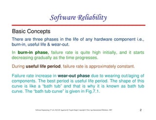
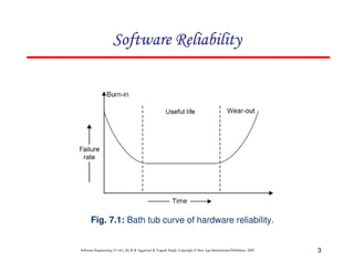
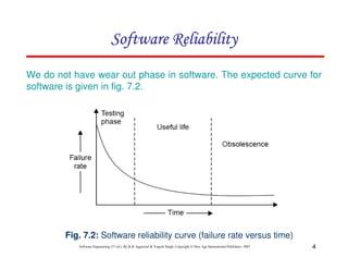
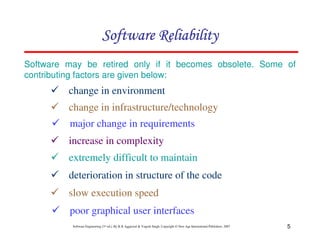
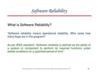

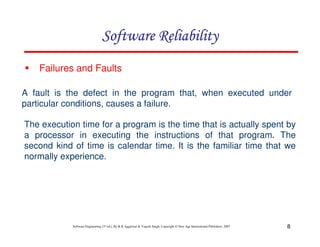
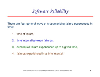
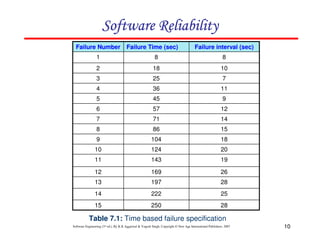
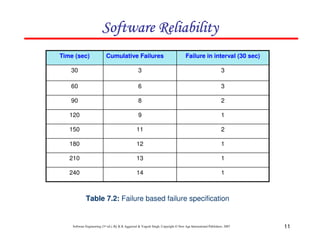
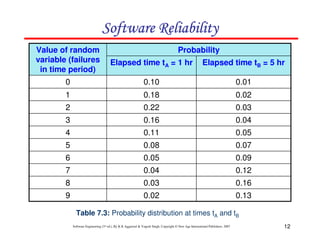
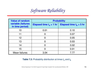
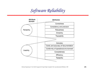
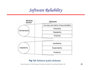
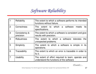
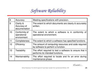
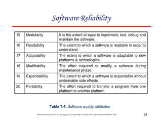
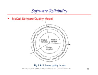

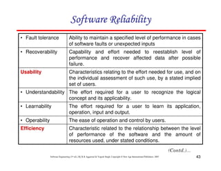
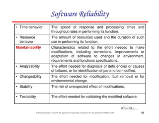
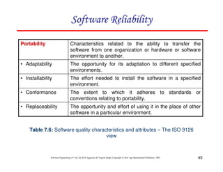
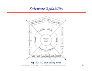
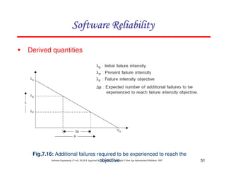
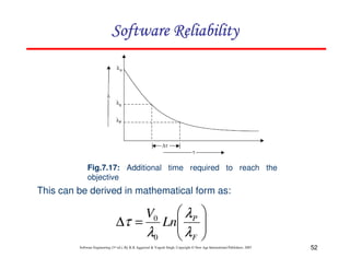

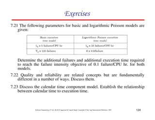
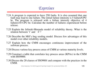
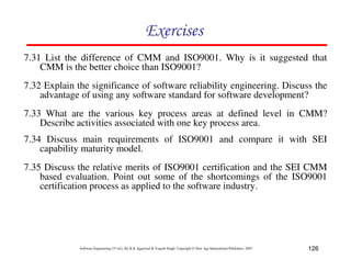

The document discusses concepts related to software reliability. It describes how software reliability is modeled using a "bathtub curve" with two phases - an initial high failure rate period and a useful life period with an approximately constant failure rate. The document defines software reliability and discusses factors that influence it like faults in the software and the execution environment. It also outlines various ways of characterizing software failures over time and presents models of failure probability distributions. Finally, it discusses uses of reliability studies and defines software quality in terms of attributes like reliability, correctness and maintainability.


![[slides] Software Engineering Third Edition - Aggarwal, Singh.pdf](https://cdn.slidesharecdn.com/ss_thumbnails/slidessoftwareengineeringthirdedition-aggarwalsingh-230615025923-02cadfc5-thumbnail.jpg?width=640&height=640&fit=bounds)