1. The document describes steps to create agro-climatic zones of Tanzania using GIS by analyzing temperature, rainfall, and evapotranspiration data. 2. Key steps include converting vector data to raster, calculating moisture availability, classifying temperature and moisture zones, and combining the zones to produce the final agro-climatic map. 3. Models are created in GIS software to automate the process and allow easy reproduction of the analysis.

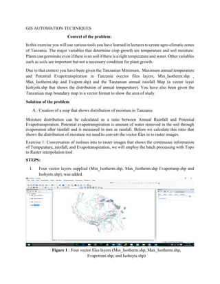
1. GIS AUTOMATION TECHNIQUES
Context of the problem:
In this exercise you will use various tools you have learned in lectures to create agro-climatic zones
of Tanzania. The major variables that determine crop growth are temperature and soil moisture.
Plants can germinate even if there is no soil if there is a right temperature and water. Other variables
such as soils are important but not a necessary condition for plant growth.
Due to that context you have been given the Tanzanian Minimum, Maximum annual temperature
and Potential Evapotranspiration in Tanzania (vector files layers, Min_Isotherm.shp ,
Max_Isotherm.shp and Evapotr.shp) and the Tanzanian annual rainfall Map (a vector layer
Isohyets.shp that shows the distribution of annual temperature). You have also been given the
Tanzanian map boundary map in a vector format to show the area of study.
Solution of the problem
A. Creation of a map that shows distribution of moisture in Tanzania
Moisture distribution can be calculated as a ratio between Annual Rainfall and Potential
Evapotranspiration. Potential evapotranspiration is amount of water removed in the soil through
evaporation after rainfall and is measured in mm as rainfall. Before we calculate this ratio that
shows the distribution of moisture we need to convert the vector files in to raster images.
Exercise 1: Conversation of isolines into to raster images that shows the continuous information
of Temperature, rainfall, and Evapotranspiration, we will employ the batch processing with Topo
to Raster interpolation tool.
STEPS:
I. Four vector layers supplied (Min_Isotherm.shp, Max_Isotherm.shp Evapotranp.shp and
Isohyets.shp), was added.
Figure 1 : Four vector files layors (Min_Isotherm.shp, Max_Isotherm.shp,
Evapotrant.shp, and Isoheyts.shp)

2. II. By opening the attribute table of each layer identification of the field that contains data can
be done (the temperature fields are given in the Fahrenheit units and the rainfall and
evapotranspiration in mm). The data value fields will be used to create the raster layers)
III. To convert vector to raster, Spatial Analyst tool>> Interpolation>> then Right Click Top
to Raster and Select Batch. Batch widow was opened and add Min_Isotherm.shp,
Max_Isotherm.shp, Evapotranp.shp and Isohyets.shp
Figure 2: Batch processing window
IV. Validating the data button before Clicking OK to run the batch processing. Check Values
also generates output dataset names. The Check Values button validates the entire batch
grid's content. Check Values also generates output dataset names.
V. After the batch is completed running four files will be produced and displayed as below:

3. ann_rain 1
min_temp
max_temp evs_temp
Figure 3: Raster display of four output layers ann_rain for isohytes Min_Temp for
Min_Isotherm.shp output, Max_temp for Max_Isotherm output and Evp_Trans for
Evapotransp.shp output

4. Figure4: batch processed display

5. Exercise 2: Creating the moisture distribution map as ration of Rainfall and
Evapotranspiration.
This operation was done by simple Math and Divide Tool when the Rainfall is divided by
evapotranspiration, the process that is known as image rationing. But also can be run using the
image calculator. We will use the image calculator although the equation is not complicated.
STEPS:
I. Open Arc Map >> Click a toolbox >> spatial analyst >> Map Algebra >> Raster calculator,
Raster Calculator was opened:
II. Following formula was entered “Ann_Rain” / “Evp_Trans” implying annual rainfall
divide by potential evapotrasipitation, the output file Moist_Av i.e., moisture availability
was assigned.
III. Click OK. Raster Calculator run and the Moisture availability raster file (Moist_Av)
produced. As per below display
Figure 5: Moisture Availability

6. Exercise 3: Production of Agro -climate zone of Tanzania
Agro-climatic zone is an important concept for agricultural planning. The concept is used to
identify regions suitable for particular crop production. Agro climatic zones for any particular
place can be determined by the combination of moisture availability and temperature zones.
Challenge 1: Produce the average annual temperature using a step by step procedure, show the
procedure and produce the result.
STEPS:
I. Image calculator in the Arc Map was opened and entering the following
formula((((Min_Temp + Max_Temp)/2)-32)*5)/9. This is a complicated formula that
calculates average annual temperature in 0C from the Mean annual Minimum Temperature
and Maximum Temperature in Fahrenheit.
II. Formula was entered by clicking the Files and the operators in the image calculator.
III. Output Five was called Av_An_T
Figure 6: Average Annual temperature in 0C

7. There in the previous steps we have produced the average annual temperature Av_An_T and the
moisture availability Moist_Av which need to be zoned and combined to produce agro climate
zones:
Exercise 3.1 Creating a moisture availability zones and Average annual temperature zone
First the temperature zone model was created. The model classifies the average Annual
temperature Av_An_T into zones using Table 2 provided and then clip the temperature zone to
Tanzania Country boundary
Steps:
I. In ArMap, Click on Modeler builder window was opened
II. Drag and drop Av_An_T on Model builder Window >> Select the file >> Click Add in the
Add data Window, the oval shaped circle in the Model Builder Window labeled Av_An_T
appeared
III. Then reclassify tool was found by click on the tool box (Spatial Analyst Tools >> Reclass
>> Reclassify) and drag and drop the tool on the model builder window
IV. The path was changed by Double Click on the Output Raster and change name from the
default folder to working folder and call the output raster file Temp_Zones.
V. The oval cycle Av_An_T was connected to Reclassify box, by clicking on the connect
tool and click on the Av_An_T oval cycle and move the magic wand that appears to
Reclassify box, and then select input raster
VI. The reclassify tool was opened by Double Click on the Reclassify box >> Change the
values in the Reclassification window to use the values in Table 2>> Reverse the New
Values. Such action will reverse the values such that low temperature zone are assigned
low value code and high temperature high value codes.
VII. Then raster was clipped by Open Tool box again >> Data Management >> Raster >> Raster
Possessing >> Clip, Drag and drop the Clip Tool on the Model Builder Window
VIII. The Output Temp_Zones was connected from Reclassify to Clip tools using a connect
tool. The tool changed the color to show that it has input
IX. Double click the Clip Tool to open the input window, Add Tz_Boundary to Output extent
(optional), Check the box, Use the Input Feature For Clipping Geometry (Optional), Write
Tz_Temp_Zones for Output raster
X. Click Ok to return to the model builder Window.
XI. Click on Auto Layout, The four blue and green boxes icon on the model builder window
toolbar. After inputting of all information your mode will look as follows:

8. Figure 6: Mode Builder Window toolbar for tz_temp_zone
Then click run on model to results the map display as seen in attached below:

9. Figure 7: Tanzania temperature Zones Map
By repeating the previous steps on exercise 3.1 above the below model was created and run to
produce Tanzania moisture availability map
Figure 8: Mode Builder Window toolbar for tz_moist_zone

10. Figure 9: Running the model completed
Figure 10: Tanzania moist zones Map

11. Exercise 3.1.1: Saving the Model.
Model you can be saved and reused. The Model is always saved in the toolbox. To serve the model
there are series of steps adding toolbox and save the model in the toolbox created. The model was
saved as moist zone and can be rerun to other analysis. It displayed as per below snapshot:
Figure 11: Saved Model

12. Figure 12: Moisture Zone availability Model
Exercise 3.2 Creation of Agro climatic Zone from Moisture availability zone and Temperature
Zone.
Steps:
1. By using batch processing of model builder both Tz_Temp_Zones and Tz_Moist_Zones
were converted to vector (Use the Tool Raster to Polygon)
Figure 13: Temperature polygon map produced

13. Figure 14: Moisture polygon map produced
2. Union Tool from Geoprocessing was used to combine the 2 vectors produced in Step 1
above and named Tz_Ag_Z. (The Single vector layer with a tables containing the
Temperature and Vector Values was produced and displayed as per below snapshot)
Figure 15: TZ_AG_Z map (Union of two polygon)
3. By studying the GRIDCODE and GRIDCODE_1 Fields, these are the values of the
Temperature zones and Field Zones, if the Value of GRIDCODE is 0 and the Values of
GRIDCODE_1 is any other value and vice versa it means those rows have no combination
of temperature zones and moisture availability zones. Therefore, they do not produce
Agro-climate Zone therefore we need to delate them and remain with row that have
GRIDCODE and GRIDECODE_1values other than 0.

14. Figure 16: Temperature zones and Field Zones
Challenge 3: Write a SQL statement to select All values with GRIDCODE value 0 and
GRIDECODE_1values 0
1. Start editor was started and select the GRIDCODE and GRIDECODE_1 with values 0 and
delete them ( by use of the SQL Tool, Query by attribute)
2. After deleting rows with GRIDCODE value 0 and GRIDECODE_1values 0 stop editing
and serve edits. The below tables were produced:

15. Figure 17: SQL Tool, Query by attribute
Figure 18: After deleting rows with GRIDCODE value 0 and GRIDECODE_1values 0 (Agro
climatic Zones of Tanzania (FID)

16. 3. FID in the map was visualized to produce The Tanzanian Agro Climate Zone Map. (It is
not possible to symbolize FID in ArcGIS. Therefore New Field was crated with the FID
Values)
4. This was done by Add Field and Call it TzAgClZ
5. Then Populate TzAgClZ Field with FID result by right clinking of the Field and Select
Field Calculator>>formula [FID] *1 was entered in the field calculator window, then OK
(The FID Valued duplicated in the TzAgClZ Field.)
6. Then Tz_Ag_Z was visualized using the Unique Value, and TzAgClZ Field was chosen
as the input values. (A map of Tanzania Agro climate Map displayed as seen in attached
below snapshot)
7. The Map was labeled with the Values of both GRIDCODE and GRIDECODE_1 to see the
moisture and Temperature combination of each zone.
Figure 19: The map showing moisture and Temperature combination of each zone

17. Challenge 4: Create a Model that produce Agro climate Zones using all steps in this practical.
Figure 20: Overall Agro climate Zones