1. Technical Note
Stratagene Mx3000P® QPCR System
Real-Time PCR Run Setup Instructions
for qBiomarker Copy Number PCR Arrays
Before the Experiment
 Please make sure the real-time PCR instrument is working properly. Refer to the manufacturer’s Installation and
Maintenance manual if needed.
Creation of PCR Protocol Template
1)
2)
3)
4)
Open the Stratagene MxPro QPCR Software on the computer that is con nected to the Stratagene Mx3000P
instrument. The New Options dialog box for an experiment will appear.
Select Real-time: SYBR® Green (with Dissociation Curve) and click OK. The new plate document will
appear.
On the top panel of the plate document, select Mx3000P (4 filter set plate).
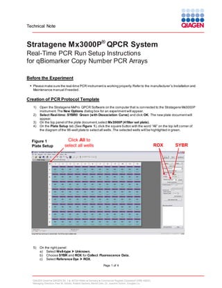
On the Plate Setup tab (See Figure 1), click the square button with the word “All” on the top left corner of
the diagram of the 96-well plate to select all wells. The selected wells will be highlighted in green.
Figure 1
Plate Setup
5)
Click All to
select all wells
ROX
On the right panel:
a) Select Well-type  Unknown.
b) Choose SYBR and ROX for Collect Fluorescence Data.
c) Select Reference Dye  ROX.
Page 1 of 4
QIAGEN GmbH  QIAGEN Str. 1  40724 Hilden  Germany  Commercial Register Düsseldorf (HRB 45822)
Managing Directors: Peer M. Schatz, Roland Sackers, Bernd Uder, Dr. Joachim Schorr, Douglas Liu
SYBR

2. Technical Note
6)
Click Next to go to the Thermal Profile Setup tab (See Figure 2). In the Application Segment panel to
the right, click Normal 2 Step. To change the default setting for the thermal profile, click directly on the
number that needs to be changed. Adjust the parameters to reflect the following:

Segment 1

Temperature: 95°C

Time: 10:00

Segment 2 (3 Steps, 40 cycles)

Step 1: 94°C, 00:15

Step 2: 60°C, 01:00, Endpoints Data Collection Marker

Segment 3 (default melt curve)

All Points Data Collect Marker must be present between Step 2 and Step 3
Figure 2
Thermal Profile Setup End Point Data
Collection Marker
7)
All Point Data
Collection Marker
Normal 2 Step
Then select File  Save As to save the template file. Save the file under the filename
“CopyNum_PCR_Array_ Mx3000P.mxp”.
Performing Real-Time PCR Detection
1)
Check to verify that the power status indicator (the lower LED on the front of the instrument) is lit and the
Ready status indicator (the upper LED) is continuously lit (glowing green). A blinking Ready status
indicator indicates an experiment is already in process; if the Ready status indicator is off, the instrument is
not available or ready to run an experiment.
Page 2 of 4
QIAGEN GmbH  QIAGEN Str. 1  40724 Hilden  Germany  Commercial Register Düsseldorf (HRB 45822)
Managing Directors: Peer M. Schatz, Roland Sackers, Bernd Uder, Dr. Joachim Schorr, Douglas Liu

3. Technical Note
2)
3)
4)
5)
6)
Ensure the reaction mix in each well of your reaction plate is free of any bubbles and positioned at the
bottom of the well. If not, centrifuge the plate at ~1000 g for 1 mins.
Open the door located on the front of the instrument by sliding it all the way to the top. To expose the
thermal block, pull forward on the hot-top handle and lift the hot-top up and away from the thermal block.
Place your plate in the plate holder with the last row (row H) facing front. Well A1 should be positioned at
the top-left corner of the thermal block. Make sure the plate is properly aligned in the holder. Close the hottop assembly by pressing down the hot-top and pushing the handle back into its original place. Slide down
the door to close.
Open the Stratagene MxPro QPCR Software. Click Cancel when the New Experiment Options dialog box
appears.
Select File  Open. Load the CopyNum_PCR_Array_ Mx3000P.mxp file. This will load the previously
saved setup to the new plate document. Save the new document under a new filename.
Click Start Run to begin the PCR run. Wait for about 30 seconds for the initial priming. The estimated run
time will then appear on the screen.
After the PCR Run
1)
2)
3)
4)
Select Analysis on the top panel of the plate docum ent page and choose the Analysis Selection/Setup
page. Click the square button with the word “All” on the top left corner of the diagram of the 96-well plate to
select all wells. The selected wells will be colored in green.
Select the Results page. On the right panel, choose Amplification plots for Area to analyze. Select 40 for
Last cycle. Select Fluorescence  dRn. Then follow the procedures below to calculate the threshold cycle
(Ct) for each well (See Figure 3):
(We highly recommend manually setting the Baseline and Threshold Value)
a. To determine the baseline, use the Linear View of the amplification plots. Double click one of the
axes. The window for Graph Properties will appear. For both Y and X-Axes, select Lo -> Hi for
Orientation and Use Automatic Limits. Select Linear Scale for Y-Axis and also for X-Axis. Then
click OK. With the linear plots, determine the cycle number at which the earliest amplification can
be seen. Select in the top menu Options  Analysis Term Settings. Set the Non-adaptive
baseline to start from cycle number 2 through two cycle values before the earliest visible
amplification. Click OK.
b. To define the Threshold Value, use the Log View of the amplification plots. Open the Graph
Properties window by double clicking one of the axes as above. Select Log Scale for Y-Axis.
Then click OK. With the log plots, place the threshold line above the background signal but within
the lower third of the linear phase of the amplification plot.
Once C T values have been determined, s elect Text Report in Area to analyze to display the results. On
the right panel, select to display the Column for Well, Well type, Threshold, CT and Tm Product 1 for
each well. In Assays Shown box at the bottom of the screen, deselect the ROX button and make sure the
SYBR button is selected so that only the data for SYBR Green will be displayed in the text report.
To export the result to an Excel spreadsheet, select File  Export Text Report  Export Text Report to
Excel and save the file as a Microsoft Excel file.
Page 3 of 4
QIAGEN GmbH  QIAGEN Str. 1  40724 Hilden  Germany  Commercial Register Düsseldorf (HRB 45822)
Managing Directors: Peer M. Schatz, Roland Sackers, Bernd Uder, Dr. Joachim Schorr, Douglas Liu

4. Technical Note
Figure 3: Setting the baseline and threshold
values View
Linear
Set the baseline
from cycle number
2 through tw o cycle
values before the
earliest visible
amplification
Earliest amplification at cycle #9
Log View
Linear Phase
Set the threshold above the background signal but
w ithin the low er third of the linear phase of the
amplification plot
Page 4 of 4
QIAGEN GmbH  QIAGEN Str. 1  40724 Hilden  Germany  Commercial Register Düsseldorf (HRB 45822)
Managing Directors: Peer M. Schatz, Roland Sackers, Bernd Uder, Dr. Joachim Schorr, Douglas Liu