1. 5 | P r o c e s s O p t i m i z a t i o n o f G r o o v e D i a m e t e r T u r n i n g
1. Problem Identification
The first step in the project was the problem identification step. In this step, the problem was
defined and all available statistical data collected to help decide the course of action.
1.1 Problem Definition
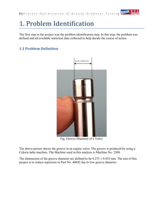
Fig. Groove Diameter of a Valve
The above picture shows the groove in an engine valve. The groove is produced by using a
Celoria lathe machine. The Machine used in this analysis is Machine No. 2308.
The dimensions of the groove diameter are defined to be 4.275 ± 0.025 mm. The aim of this
project is to reduce rejections in Part No. 40692 due to low groove diameter.
4.275 ± 0.025 mm
2. 6 | P r o c e s s O p t i m i z a t i o n o f G r o o v e D i a m e t e r T u r n i n g
2. Observation
Once the basic problem has been defined, it is important to critically observe the processes to
understand where the problem originates from. For this purpose, several quality control tools are
used.
2.1Process Flow Diagram
The process flow diagram represents the various machining operations performed on the part.
The advantage of studying process flow diagrams is that the various operations can be analysed
and the exact point of problem can be easily identified. It also helps in relating various
operations in the manufacturing line enabling us to identify sources of problems in operations
that are performed before the operation under study.
The problem in our study, low groove diameter occurs in the “Groove Diameter and Chamfer”
step. The operation preceding the groove diameter turning is the stress relieving step. From the
flow diagram, it is also clear that the centre less grinding operation will directly have an impact
on groove turning, since material removal happens in the region where the groove diameter is to
be turned. Thus, any variation in dimension at the end o the centre less grinding operation will
directly contribute towards dimensional variations in the groove diameter.
3. 7 | P r o c e s s O p t i m i z a t i o n o f G r o o v e D i a m e t e r T u r n i n g
2.2Process Capability Chart
The input of a process usually has at least one or more measurable characteristics that are used to
specify outputs. These can be analyzed statistically; where the output data shows a normal
distribution the process can be described by the process mean (average) and the standard
deviation.
A process needs to be established with appropriate process controls in place. A control
chart analysis is used to determine whether the process is "in statistical control". If the process is
not in statistical control then capability has no meaning. Therefore the process capability
involves only common cause variation and not special cause variation.
A batch of data needs to be obtained from the measured output of the process. The more data that
is included the more precise the result, however an estimate can be achieved with as few as 17
data points. This should include the normal variety of production conditions, materials, and
people in the process. With a manufactured product, it is common to include at least three
different production runs, including start-ups.
The output of a process is expected to meet customer requirements, specifications, or
product tolerances. Engineering can conduct a process capability study to determine the extent to
which the process can meet these expectations.
The ability of a process to meet specifications can be expressed as a single number using
a process capability index or it can be assessed using control charts. Either case requires running
the process to obtain enough measurable output so that engineering is confident that the process
is stable and so that the process mean and variability can be reliably estimated. Statistical process
control defines techniques to properly differentiate between stable processes, processes that are
drifting (experiencing a long-term change in the mean of the output), and processes that are
growing more variable. Process capability indices are only meaningful for processes that are
stable (in a state of statistical control).
A process capability study was conducted for the part number under study. 50 samples were
collected from the groove diameter operation and checked for their dimensions. A capability
study of the data was performed. The Process Capability chart and the inferences drawn from it
are expressed as follows.
4. 8 | P r o c e s s O p t i m i z a t i o n o f G r o o v e D i a m e t e r T u r n i n g
The process capability chart of the groove diameter turning operation is shown above. The
sample population was observed to have a mean of 4.2638 mm. The curve shows that the values
of the diameters lean towards the lower specification limit of 4.25 mm and the mean is shifted
towards the LSL from the 4.275 mm mark. 4 samples from the population were observed to lie
outside the specification limits – 3 below the LSL and 1 above the USL.
The overall process capability was observed to be 0.33 which indicates that there is wide scope
for improvement in the operation.
2.3 Response Analysis Table
The Response analysis table is used to check the conformance of existing procedures to
established quality levels. This is done by taking a sample population and comparing it with the
specifications.
S.No Response
Is there
Spec
If so What is
the Spec
Is it being
monitored & how
What Is actual
Is there an actual or
potential difference
Action Plan
1
Groove Diameter
Low
Yes 4.25~4.30 mm
Yes & 100% by
Snap Gauge
50 Nos checked
(4.232~4.323mm)
0.041mm CAT
RESPONSE ANALYSIS TABLE
5. 9 | P r o c e s s O p t i m i z a t i o n o f G r o o v e D i a m e t e r T u r n i n g
3.ANALYSIS
Once the basic data is obtained, it is important to critically examine the data and collect information
that helps identify the root cause of the problem. The Analysis step involves studying the process and
parameters using various statistical tools and identifying the chief contributors to the defect. Several
tools were used as a part of this project and they have been described in the following pages
3.1Fishbone diagram
Ishikawa diagrams (also called fishbone diagrams, or herringbone diagrams, cause-and-
effect diagrams, or Fishikawa) are causal diagrams that show the causes of a certain event --
created by Kaoru Ishikawa (1990).Common uses of the Ishikawa diagram are product design and
quality defect prevention, to identify potential factors causing an overall effect. Each cause or
reason for imperfection is a source of variation. Causes are usually grouped into major categories
to identify these sources of variation. The categories typically include:
Man: Anyone involved with the process
Methods: How the process is performed and the specific requirements for doing it, such as
policies, procedures, rules, regulations and laws
Machines: Any equipment, computers, tools etc. required to accomplish the job
Materials: Raw materials, parts, pens, paper, etc. used to produce the final product
Measurements: Data generated from the process that are used to evaluate its quality
Environment: The conditions, such as location, time, temperature, and culture in which the
process operates
A fishbone diagram was made for the problem of low groove diameter. It is shown below.
Groove Dia
Size Variation
MAN
METHOD
Dwell time high
MACHINE
Feed Rate Low
MATERIAL
Hyd oil Temperature High
Dwell time low
Tool grinding not proper
Feed Rate High
Wrong setting by operator
Spindle RPM
Collet worn out
Slide movement
Repeatability
Stem Hardness High
Improper Gauge size
Stem Hardness Low
Stem Runout High
6. 10 | P r o c e s s O p t i m i z a t i o n o f G r o o v e D i a m e t e r T u r n i n g
3.2 Cause Analysis Table
Cause Analysis Table is a tool for problem solving aimed at identifying the root causes of
problems or events.
Cause Analysis is any structured approach to identifying the factors that resulted in the nature,
the magnitude, the location, and the timing of the outcomes (consequences) of one or more
defects in order to identify what behaviors, actions, inactions, or conditions need to be changed
to prevent recurrence of similar defects and to identify the lessons to be learned to promote the
achievement of better output.
The Cause Analysis Table is predicated on the belief that problems are best solved by attempting
to address, correct or eliminate root causes, as opposed to merely addressing the immediately
obvious symptoms. By directing corrective measures at root causes, it is more probable that
problem recurrence will be prevented.
A brain storming session is held to identify the various causes of low groove diameter from the
fishbone diagram and conclude whether or not it is a factor contributing towards the defect. The
standard operation procedures, maintenance check lists and other procedural materials are
studied and data collected on standard specifications. It is then checked if the operating
parameters conform to these standard specifications and any discrepancies are documented. The
table also lists details on action to be taken on specific factors.
The Cause Analysis Table is presented on the following page.
7. 11 | P r o c e s s O p t i m i z a t i o n o f G r o o v e D i a m e t e r T u r n i n g
8. 12 | P r o c e s s O p t i m i z a t i o n o f G r o o v e D i a m e t e r T u r n i n g
3.3 Selection of Factors
From the Cause analysis, the various possible causes are obtained. Experiments were conducted
to study the contribution of each of these factors and determine if they significantly contribute to
the defect. Data of the analyzed factors is given below.
1. Feed Rate Variation
Fig. Knob for controlling Feed Rate
Feed rate variation is checked for selection as a factor by testing samples at three different feed
rates. Observe that the range of the output diameter lies below specification at 5mm/min while it
lies above the specification at 3mm/min.
S.No Diameter S.No Diameter S.No Diameter
1 4.656 1 4.310 1 4.226
2 4.686 2 4.286 2 4.254
3 4.680 3 4.268 3 4.232
4 4.688 4 4.270 4 4.266
5 4.676 5 4.300 5 4.238
6 4.654 6 4.260 6 4.250
7 4.684 7 4.268 7 4.232
8 4.676 8 4.262 8 4.246
9 4.644 9 4.265 9 4.258
10 4.680 10 4.260 10 4.234
Feed Rate =
3mm/min
Feed Rate =
4mm/min
Feed Rate =
5mm/min
9. 13 | P r o c e s s O p t i m i z a t i o n o f G r o o v e D i a m e t e r T u r n i n g
2. Hydraulic Temperature
The operations in the celoria lathe are automatically operated through hydraulic and pneumatic
systems. In such hydraulically operated systems, the hydraulic oil temperature is found to play an
important role in the accuracy and repeatability of the system. Hence, a test was performed to
check the effect of hydraulic temperature on the output. From the above observations, it is clear
that the turning operation results in precise dimensions in the presence of a chiller unit rather
than its absence.
3. Stem Hardness
In the course of the observation period, it was found that the most widely believed reason for the
low groove diameter was incorrect hardness. Hence, a population of 50 samples was analyzed for
relation of groove diameter to hardness. While hardness did not present any direct relation to the
diameter, it was still included as a factor to confirm this observation.
S. No Diameter S. No Diameter
1 4.282 1 4.238
2 4.256 2 4.236
3 4.290 3 4.238
4 4.270 4 4.242
5 4.284 5 4.248
6 4.288 6 4.302
7 4.276 7 4.288
8 4.284 8 4.272
9 4.272 9 4.280
10 4.280 10 4.276
11 4.276 11 4.290
12 4.274 12 4.268
13 4.276 13 4.300
14 4.254 14 4.262
15 4.264 15 4.265
Without ChillerWith Chiller
S. No Hardness Diameter S. No Hardness Diameter S. No Hardness Diameter
1 39 4.268 21 30 4.264 41 33 4.270
2 38 4.272 22 19 4.262 42 36 4.270
3 38 4.323 23 22 4.274 43 35 4.274
4 39 4.248 24 17 4.268 44 36 4.266
5 35 4.232 25 30 4.264 45 37 4.274
6 36 4.270 26 27 4.258 46 35 4.266
7 39 4.266 27 20 4.266 47 38 4.266
8 38 4.252 28 25 4.246 48 39 4.274
9 30 4.254 29 36 4.254 49 38 4.290
10 32 4.252 30 36 4.256 50 33 4.268
11 26 4.252 31 29 4.250
12 36 4.250 32 37 4.250
13 38 4.264 33 35 4.268
14 24 4.246 34 32 4.264
15 29 4.250 35 37 4.276
16 31 4.254 36 34 4.282
17 30 4.258 37 34 4.250
18 31 4.266 38 38 4.272
19 24 4.274 39 39 4.278
20 25 4.260 40 35 4.262
10. 14 | P r o c e s s O p t i m i z a t i o n o f G r o o v e D i a m e t e r T u r n i n g
4. Spindle RPM
According to the fundamental principles of manufacturing, spindle rpm has a direct
relation to the feed rate and work piece diameter. Hence, it was included as a factor to
check if it has an impact on the groove diameter.
5. Dwell Time
The dwell time of the turning operation decides the amount of material removed.
Thereby, it can contribute to variations in the groove diameter. Higher dwell time
removes more material than necessary, while with lower dwell times, lesser material is
removed. This is shown in the following data obtained at different dwell times.
Fig. Dwell Time Adjustment Knob
S.No Diameter S.No Diameter
1 4.294 1 4.244
2 4.242 2 4.242
3 4.256 3 4.238
4 4.298 4 4.242
5 4.25 5 4.204
6 4.252 6 4.252
7 4.254 7 4.236
8 4.262 8 4.244
9 4.292 9 4.246
10 4.282 10 4.238
11 4.254 11 4.254
12 4.246 12 4.242
13 4.242 13 2.238
14 4.288 14 4.246
15 4.264 15 4.248
Speed=2100 rpm Speed=1600rpm
S. No S. No
1 4.238 1 4.262
2 4.246 2 4.272
3 4.250 3 4.266
4 4.246 4 4.254
5 4.242 5 4.248
6 4.250 6 4.286
7 4.248 7 4.474
8 4.252 8 4.280
9 4.244 9 4.276
10 4.246 10 4.274
11 4.234 11 4.264
12 4.238 12 4.270
13 4.242 13 4.268
14 4.236 14 4.282
15 4.240 15 4.276
Dwell Time 0.2 s Dwell Time 0.4s
11. 15 | P r o c e s s O p t i m i z a t i o n o f G r o o v e D i a m e t e r T u r n i n g
Based on the information presented in the cause analysis table, the following factors were
selected for further evaluation.
3.4 Assignment of Factor Levels
Once the factors have been identified, values must be assigned for various levels of the factor.
For every factor, a degree of freedom is 2 while for every interaction, the degree of freedom is 4.
Based on this, the minimum number of experiments required is 27. Thus L2734
is chosen for the
Design of experiments.
FACTOR
CODE
FACTORS
A Spindle RPM
B Hydraulic Temperature
C Feed Rate Variation
D Dwell Time
E Stem Hardness
12. 16 | P r o c e s s O p t i m i z a t i o n o f G r o o v e D i a m e t e r T u r n i n g
3.5 Linear Graph
A linear graph is drawn that assigns columns to the various selected factors and presents the
relation between them. The linear graph is shown below.
3.6 Orthogonal Array & Experimental Layout
In order to conduct the experiments, it is important to use all 3 levels of all the five factors in all
possible combinations. For a large number of factors and experiments, this may get tedious and
take a lot of human effort and time. To make it simpler to include all possible combinations, an
orthogonal array appropriate for the given number of experiments is used.
The experimental layout presents the value of each factor for each of the experiments that need
to be conducted. The experimental layout is prepared with the help of the orthogonal arrays.
Each experiment has a different combination of factors at different layers.
(Refer Appendix 2 and Appendix 3)
13. 17 | P r o c e s s O p t i m i z a t i o n o f G r o o v e D i a m e t e r T u r n i n g
2 1 5 4 9
Exp A B C D E
1 1 1 1 1 1
2 1 1 2 1 2
3 1 1 3 1 3
4 2 1 1 2 2
5 2 1 2 2 3
6 2 1 3 2 1
7 3 1 1 3 3
8 3 1 2 3 1
9 3 1 3 3 2
10 1 2 1 3 2
11 1 2 2 3 3
12 1 2 3 3 1
13 2 2 1 1 3
14 2 2 2 1 1
15 2 2 3 1 2
16 3 2 1 2 1
17 3 2 2 2 2
18 3 2 3 2 3
19 1 3 1 2 3
20 1 3 2 2 1
21 1 3 3 2 2
22 2 3 1 3 1
23 2 3 2 3 2
24 2 3 3 3 3
25 3 3 1 1 2
26 3 3 2 1 3
27 3 3 3 1 1
Table. Orthogonal Array Table
14. 18 | P r o c e s s O p t i m i z a t i o n o f G r o o v e D i a m e t e r T u r n i n g
2 1 5 4 9
A B C D E
1 Spindle RPM@1600
Hydraulic
Temperature@2
4
Feed Rate
Variation@5
Dwell
Time@10
Hardness@14~
20
2 Spindle RPM@1600
Hydraulic
Temperature@2
4
Feed Rate
Variation@6
Dwell
Time@10
Hardness@24~
30
3 Spindle RPM@1600
Hydraulic
Temperature@2
4
Feed Rate
Variation@7
Dwell
Time@10
Hardness@32~
38
4 Spindle RPM@2100
Hydraulic
Temperature@2
4
Feed Rate
Variation@5
Dwell
Time@20
Hardness@24~
30
5 Spindle RPM@2100
Hydraulic
Temperature@2
4
Feed Rate
Variation@6
Dwell
Time@20
Hardness@32~
38
6 Spindle RPM@2100
Hydraulic
Temperature@2
4
Feed Rate
Variation@7
Dwell
Time@20
Hardness@14~
20
7 Spindle RPM@2100
Hydraulic
Temperature@2
4
Feed Rate
Variation@5
Dwell
Time@30
Hardness@32~
38
8 Spindle RPM@2100
Hydraulic
Temperature@2
4
Feed Rate
Variation@6
Dwell
Time@30
Hardness@14~
20
9 Spindle RPM@2100
Hydraulic
Temperature@2
4
Feed Rate
Variation@7
Dwell
Time@30
Hardness@24~
30
10 Spindle RPM@1600
Hydraulic
Temperature@2
9
Feed Rate
Variation@5
Dwell
Time@30
Hardness@24~
30
11 Spindle RPM@1600
Hydraulic
Temperature@2
9
Feed Rate
Variation@6
Dwell
Time@30
Hardness@32~
38
12 Spindle RPM@1600
Hydraulic
Temperature@2
9
Feed Rate
Variation@7
Dwell
Time@30
Hardness@14~
20
13 Spindle RPM@2100
Hydraulic
Temperature@2
9
Feed Rate
Variation@5
Dwell
Time@10
Hardness@32~
38
14 Spindle RPM@2100
Hydraulic
Temperature@2
9
Feed Rate
Variation@6
Dwell
Time@10
Hardness@14~
20
15 Spindle RPM@2100
Hydraulic
Temperature@2
9
Feed Rate
Variation@7
Dwell
Time@10
Hardness@24~
30
16 Spindle RPM@2100
Hydraulic
Temperature@2
9
Feed Rate
Variation@5
Dwell
Time@20
Hardness@14~
20
17 Spindle RPM@2100
Hydraulic
Temperature@2
9
Feed Rate
Variation@6
Dwell
Time@20
Hardness@24~
30
18 Spindle RPM@2100
Hydraulic
Temperature@2
9
Feed Rate
Variation@7
Dwell
Time@20
Hardness@32~
38
19 Spindle RPM@1600
Hydraulic
Temperature@3
4
Feed Rate
Variation@5
Dwell
Time@20
Hardness@32~
38
20 Spindle RPM@1600
Hydraulic
Temperature@3
4
Feed Rate
Variation@6
Dwell
Time@20
Hardness@14~
20
21 Spindle RPM@1600
Hydraulic
Temperature@3
4
Feed Rate
Variation@7
Dwell
Time@20
Hardness@24~
30
22 Spindle RPM@2100
Hydraulic
Temperature@3
4
Feed Rate
Variation@5
Dwell
Time@30
Hardness@14~
20
23 Spindle RPM@2100
Hydraulic
Temperature@3
4
Feed Rate
Variation@6
Dwell
Time@30
Hardness@24~
30
24 Spindle RPM@2100
Hydraulic
Temperature@3
4
Feed Rate
Variation@7
Dwell
Time@30
Hardness@32~
38
25 Spindle RPM@2100
Hydraulic
Temperature@3
4
Feed Rate
Variation@5
Dwell
Time@10
Hardness@24~
30
26 Spindle RPM@2100
Hydraulic
Temperature@3
4
Feed Rate
Variation@6
Dwell
Time@10
Hardness@32~
38
27 Spindle RPM@2100
Hydraulic
Temperature@3
4
Feed Rate
Variation@7
Dwell
Time@10
Hardness@14~
20
Exp
Table. Experimental Layout
16. 20 | P r o c e s s O p t i m i z a t i o n o f G r o o v e D i a m e t e r T u r n i n g
From the above table, the factors that contribute the maximum extent to variation in
the groove diameter are found to be dwell time and feed rate, in that order.
3.8 Best Combination of Factors
Based on the obtained data on diameters of the valves, the following factors have
been selected as the best combination of factors.
Best combination
A2 Spindle RPM@2100
B2 Hydraulic Temperature@29
C3 Feed Rate Variation@7
D3 Dwell Time@30
E3 Hardness@32~38
DOF SS MS F Cal F Tab
Is it
Significa
nt
%
Contribu
tion
A Spindle RPM 2 0.019 0.010 0.624 3.041 No
B Hyd Temperature 2 0.073 0.036 2.369 3.041 No
C Feed Rate variation 2 1.117 0.558 36.420 3.041 Yes 2.82
D Dwell Time 2 33.345 16.673 1087.391 3.041 Yes 86.43
E Hardness 2 0.001 0.001 0.041 3.041 No
AC 4 0.054 0.013 0.878 2.417 No
BC 4 0.066 0.016 1.069 2.417 No
CE 4 0.085 0.021 1.379 2.417 No
247 3.787 0.015
269 38.546 89.25
Error
Total
Source
of Variation
17. 21 | P r o c e s s O p t i m i z a t i o n o f G r o o v e D i a m e t e r T u r n i n g
4. Check Result
4.1 Confirmation Trial
A confirmation trial was conducted for 50 numbers using the combination of factors selected
above. The following data was obtained.
S.No Groove Diameter
1 4.270
2 4.284
3 4.281
4 4.265
5 4.285
6 4.281
7 4.277
8 4.290
9 4.280
10 4.285
11 4.283
12 4.276
13 4.274
14 4.290
15 4.269
16 4.290
17 4.280
18 4.290
19 4.281
20 4.282
21 4.287
22 4.265
23 4.275
24 4.270
25 4.280
26 4.276
27 4.270
28 4.275
29 4.280
30 4.280
31 4.285
32 4.275
33 4.270
34 4.290
35 4.280
36 4.287
37 4.275
38 4.267
39 4.268
40 4.265
41 4.281
42 4.285
43 4.272
44 4.276
45 4.278
46 4.285
47 4.287
48 4.290
49 4.272
50 4.274
18. 22 | P r o c e s s O p t i m i z a t i o n o f G r o o v e D i a m e t e r T u r n i n g
4.2 Process Capability Chart
The process capability for the operation was obtained to be as follows.
Before After
Cp 0.34 1.14
Cpk 0.30 1.01
19. 23 | P r o c e s s O p t i m i z a t i o n o f G r o o v e D i a m e t e r T u r n i n g
5.Standardisation
Once the best combination of factors has been determined and validated, it is important to
implement it in the shop floor. For this purpose, standardization is performed and the changed
parameters are incorporated into the standard operating procedure as follows.
20. 24 | P r o c e s s O p t i m i z a t i o n o f G r o o v e D i a m e t e r T u r n i n g
6.Conclusion
The factors contributing to low groove diameter in part no. 40692 were studied and determined.
A Design of Experiments exercise was carried out to determine the best combination of factors.
The best combination of factors was found to be
Best combination
A2 Spindle RPM@2100
B2 Hydraulic Temperature@29
C3 Feed Rate Variation@7
D3 Dwell Time@30
E3 Hardness@32~38
Based on these factors, a confirmation trial was conducted.
The process capability of the operation improved, hence validating the results of the
experimental results.
21. 25 | P r o c e s s O p t i m i z a t i o n o f G r o o v e D i a m e t e r T u r n i n g
APPENDIX – 1: F Table for Alpha
22. 26 | P r o c e s s O p t i m i z a t i o n o f G r o o v e D i a m e t e r T u r n i n g
Appendix – 2: Experimental Trial Sheet
23. 27 | P r o c e s s O p t i m i z a t i o n o f G r o o v e D i a m e t e r T u r n i n g
Appendix – 3: Experimental Layout
24. 28 | P r o c e s s O p t i m i z a t i o n o f G r o o v e D i a m e t e r T u r n i n g
Bibliography
1. Dale H.Besterfiled, at., “Total Quality Management”, Pearson Education Asia,
Third Edition, Indian Reprint (2006).
2. James R. Evans and William M. Lindsay, “The Management and Control of Quality”,
6th Edition, South-Western (Thomson Learning), 2005.
3. Oakland, J.S. “TQM – Text with Cases”, Butterworth – Heinemann Ltd., Oxford, 3rd
Edition, 2003.
4. Suganthi,L and Anand Samuel, “Total Quality Management”, Prentice Hall (India)
Pvt. Ltd.,2006.
5. Janakiraman,B and Gopal, R.K, “Total Quality Management – Text and Cases”,
Prentice Hall (India) Pvt. L