This document provides an introduction to cryogenics and discusses several key topics: 1) It defines cryogenics as dealing with very low temperatures and their effects on matter, listing some common cryogenic fluids and their characteristic temperatures. 2) Heat transfer and thermal insulation methods at cryogenic temperatures are described, including differences from higher temperatures. 3) Refrigeration and liquefaction techniques for producing cryogenic fluids are briefly mentioned. 4) Cryogen storage and thermometry at low temperatures are noted as additional topics to be covered.

1. Introduction to Cryogenics
Philippe Lebrun
President of the IIR General Conference
International Institute of Refrigeration
2018

2. Contents
• Introduction
• Cryogenic fluids
• Heat transfer & thermal insulation
• Thermal screening with cold vapour
• Refrigeration & liquefaction
• Cryogen storage
• Thermometry
Ph. Lebrun Introduction to Cryogenics 2

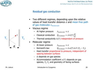
3. • 𝛋𝛠𝛖𝛐𝛓, 𝛐𝛖𝛓 το 1 deep cold [Arist. Meteor.]
2 shiver of fear [Aeschyl. Eumenid.]
• cryogenics, that branch of physics which deals with the
production of very low temperatures and their effects on matter
Oxford English Dictionary
2nd edition, Oxford University Press (1989)
• cryogenics, the science and technology of temperatures below
120 K
New International Dictionary of Refrigeration
4th edition, IIF-IIR Paris (2015)
Ph. Lebrun Introduction to Cryogenics 3

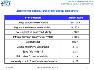
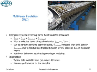
4. Characteristic temperatures of cryogens
Cryogen Triple point [K]
Normal boiling
point [K]
Critical point
[K]
Methane 90.7 111.6 190.5
Oxygen 54.4 90.2 154.6
Argon 83.8 87.3 150.9
Nitrogen 63.1 77.3 126.2
Neon 24.6 27.1 44.4
Hydrogen 13.8 20.4 33.2
Helium 2.2 (*) 4.2 5.2
(*): l Point
Ph. Lebrun Introduction to Cryogenics 4

5. Cryogenic transport of natural gas: LNG
130 000 m3 LNG carrier
with double hull
Invar® tanks hold LNG at ~110 K
Ph. Lebrun JUAS 2017 Intro to Cryogenics 5

6. Air separation by cryogenic
distillation
Capacity up to 4500 t/day LOX
LIN as byproduct
Densification, liquefaction & separation of gases
LIN & LOX
Ph. Lebrun JUAS 2017 Intro to Cryogenics 6

7. Densification, liquefaction & separation of gases
Rocket fuels
Ariane 5
25 t LHY, 130 t LOX
Space Shuttle
100 t LHY, 600 t LOX
Ph. Lebrun JUAS 2017 Intro to Cryogenics 7

8. What is a low temperature?
• The entropy of a thermodynamical system in
a macrostate corresponding to a multiplicity
W of microstates is
S = kB ln W
• Adding reversibly heat dQ to the system
results in a change of its entropy dS with a
proportionality factor T
T = dQ/dS
 high temperature: heating produces
small entropy change
 low temperature: heating produces
large entropy change
L. Boltzmann’s grave in the Zentralfriedhof,
Vienna, bearing the entropy formula
Ph. Lebrun JUAS 2017 Intro to Cryogenics 8

9. Temperature and energy
• The average thermal energy of a particle in a system in thermodynamic
equilibrium at temperature T is
E ~ kB T
kB = 1.3806 × 10−23 J.K-1
• 1 K is equivalent to ~10-4 eV or ~10-23 J thermal energy
– a temperature is « low » for a given physical process when the
corresponding average thermal energy kBT is small compared with
the characteristic energy E of the process considered
– cryogenic temperatures reveal phenomena with low characteristic
energy and enable their study and their application
Ph. Lebrun JUAS 2017 Intro to Cryogenics 9

10. Characteristic temperatures of low-energy phenomena
Phenomenon Temperature
Debye temperature of metals few 100 K
High-temperature superconductivity ~ 100 K
Low-temperature superconductivity ~ 10 K
Intrinsic transport properties of metals < 10 K
Cryopumping few K
Cosmic microwave background 2.7 K
Superfluid helium 4 2.2 K
Bolometers for cosmic radiation < 1 K
Low-density atomic Bose-Einstein condensates ~ mK
Ph. Lebrun JUAS 2017 Intro to Cryogenics 10

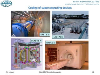
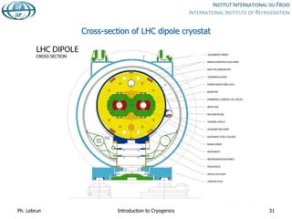
11. Useful range of liquid cryogens & critical temperature of superconductors
0 20 40 60 80 100 120 140 160 180
Oxygen
Argon
Nitrogen
Neon
Hydrogen
Helium
T [K]
Below Patm
Above Patm
Nb-Ti
Nb3Sn
Mg B2 YBCO Bi-2223
Ph. Lebrun Introduction to Cryogenics 11

12. Cooling of superconducting devices
Ph. Lebrun JUAS 2017 Intro to Cryogenics 12
LHe 1.9 K
SCHe 4.5 K
LIN ~70 K
LHe 4.2 K

13. Contents
• Introduction
• Cryogenic fluids
• Heat transfer & thermal insulation
• Thermal screening with cold vapour
• Refrigeration & liquefaction
• Cryogen storage
• Thermometry
Ph. Lebrun Introduction to Cryogenics 13

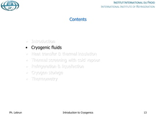
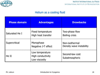
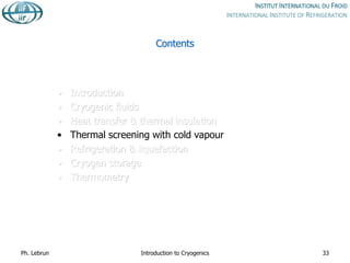
14. Properties of cryogens compared to water
Property He N2 H2O
Normal boiling point [K] 4.2 77 373
Critical temperature [K] 5.2 126 647
Critical pressure [bar] 2.3 34 221
Liq./Vap. density (*) 7.4 175 1600
Heat of vaporization (*) [J.g-1] 20.4 199 2260
Liquid viscosity (*) [mPl] 3.3 152 278
(*) at normal boiling point
Ph. Lebrun Introduction to Cryogenics 14

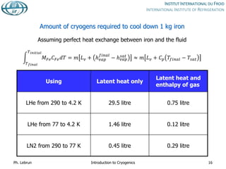
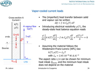
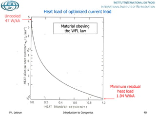
15. Vaporization of normal boiling cryogens
under 1 W applied heat load
Cryogen [mg.s-1] [l.h-1] (liquid)
[l.min-1]
(gas NTP)
Helium 48 1.38 16.4
Nitrogen 5 0.02 0.24
Ph. Lebrun Introduction to Cryogenics 15
Let ℎ be the enthalpy of the fluid
At constant pressure 𝑄 = 𝐿𝑣𝑚 with 𝐿𝑣 = ℎ𝑣𝑎𝑝 − ℎ𝑙𝑖𝑞

16. Amount of cryogens required to cool down 1 kg iron
Using Latent heat only
Latent heat and
enthalpy of gas
LHe from 290 to 4.2 K 29.5 litre 0.75 litre
LHe from 77 to 4.2 K 1.46 litre 0.12 litre
LN2 from 290 to 77 K 0.45 litre 0.29 litre
Ph. Lebrun Introduction to Cryogenics 16
Assuming perfect heat exchange between iron and the fluid
𝑇𝑓𝑖𝑛𝑎𝑙
𝑇𝑖𝑛𝑖𝑡𝑖𝑎𝑙
𝑀𝐹𝑒𝐶𝐹𝑒𝑑𝑇 = 𝑚 𝐿𝑣 + ℎ𝑣𝑎𝑝
𝑓𝑖𝑛𝑎𝑙
− ℎ𝑣𝑎𝑝
𝑠𝑎𝑡
≈ 𝑚 𝐿𝑣 + 𝐶𝑝 𝑇𝑓𝑖𝑛𝑎𝑙 − 𝑇𝑠𝑎𝑡

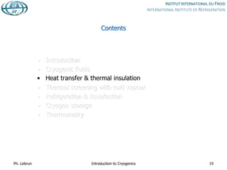
17. Phase diagram of helium
1
10
100
1000
10000
0 1 2 3 4 5 6
Temperature [K]
Pressure
[kPa]
SOLID
VAPOUR
He I
He II
CRITICAL
POINT
PRESSURIZED He II
(Subcooled liquid)
SATURATED He II
SUPER-
CRITICAL
SATURATED He I
l LINE
Ph. Lebrun Introduction to Cryogenics 17

18. Helium as a cooling fluid
Phase domain Advantages Drawbacks
Saturated He I
Fixed temperature
High heat transfer
Two-phase flow
Boiling crisis
Supercritical Monophase
Negative J-T effect
Non-isothermal
Density wave instability
He II
Low temperature
High conductivity
Low viscosity
Second-law cost
Subatmospheric
Ph. Lebrun Introduction to Cryogenics 18

19. Contents
• Introduction
• Cryogenic fluids
• Heat transfer & thermal insulation
• Thermal screening with cold vapour
• Refrigeration & liquefaction
• Cryogen storage
• Thermometry
Ph. Lebrun Introduction to Cryogenics 19

20. Typical heat transfer coefficients
at cryogenic temperatures
• Same basic processes as at
temperatures above ambiant, but
large variations in
- absolute values
- dependence on temperature
• These variations can be exploited
for
- cooling equipment
- thermal insulation of cryostats
• Particular importance of two-
phase heat transfer
Ph. Lebrun Introduction to Cryogenics 20

21. Non-linear heat transfer to liquid cryogens
Pool boiling nitrogen
~ 1.5 105 W/m2
Ph. Lebrun Introduction to Cryogenics 21

22. Non-linear heat transfer to liquid cryogens
Pool boiling helium
104 W/m2
Ph. Lebrun Introduction to Cryogenics 22

23. Heat conduction in solids
• Fourier’s law 𝑄𝑐𝑜𝑛𝑑 = 𝑘 𝑇 𝐴
𝑑𝑇
𝑑𝑥
• Thermal conductivity 𝑘 𝑇 [W/m.K]
• Integral form 𝑄𝑐𝑜𝑛𝑑 =
𝐴
𝐿 𝑇1
𝑇2
𝑘 𝑇 𝑑𝑇
• Thermal conductivity integral 𝑇1
𝑇2
𝑘 𝑇 𝑑𝑇 [W/m]
• Thermal conductivity integrals for standard
construction materials are tabulated
Ph. Lebrun Introduction to Cryogenics 23
d
x
Q c o n
T 1
T 2
S
d T
A

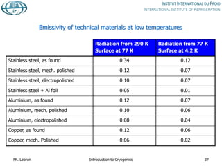
24. Thermal conductivity integrals
of selected materials [W/m]
From vanishingly low temperature
up to
20 K 80 K 290 K
OFHC copper 11000 60600 152000
DHP copper 395 5890 46100
1100 aluminium 2740 23300 72100
2024 aluminium alloy 160 2420 22900
AISI 304 stainless steel 16.3 349 3060
G-10 glass-epoxy composite 2 18 153
Ph. Lebrun Introduction to Cryogenics 24

25. Non-metallic composite
support post
with heat intercepts
5 K cooling line (SC He)
Aluminium strips to thermal
shield at 50-75 K
Aluminium intercept plates
glued to G-10 column
Ph. Lebrun Introduction to Cryogenics 25

26. Thermal radiation
• Wien’s law
– Maximum of black-body power spectrum
𝜆𝑚𝑎𝑥 𝑇 = 2898 [μm. K]
• Stefan-Boltzmann’s law
– Black body 𝑄𝑟𝑎𝑑 = 𝜎 𝐴 𝑇4
with 𝜎 = 5.67 10−12
W/m2
K4
– «Gray» body 𝑄𝑟𝑎𝑑 = 𝜀 𝜎 𝐴 𝑇4
with 𝜀 surface emissivity
– Between «gray» surfaces at temperatures 𝑇1 and 𝑇2
𝑄𝑟𝑎𝑑 = 𝐸 𝜎 𝐴 (𝑇2
4
− 𝑇1
4
)
with 𝐸 function of 𝜀1, 𝜀2 and
geometry of facing surfaces
Ph. Lebrun Introduction to Cryogenics 26
T
1 T
2 >T
1

1 
2
Q
ra
d
1
Q
ra
d
2

27. Emissivity of technical materials at low temperatures
Radiation from 290 K
Surface at 77 K
Radiation from 77 K
Surface at 4.2 K
Stainless steel, as found 0.34 0.12
Stainless steel, mech. polished 0.12 0.07
Stainless steel, electropolished 0.10 0.07
Stainless steel + Al foil 0.05 0.01
Aluminium, as found 0.12 0.07
Aluminium, mech. polished 0.10 0.06
Aluminium, electropolished 0.08 0.04
Copper, as found 0.12 0.06
Copper, mech. Polished 0.06 0.02
Ph. Lebrun Introduction to Cryogenics 27

28. Residual gas conduction
• Two different regimes, depending upon the relative
values of heat transfer distance 𝑑 and mean free path
of gas molecules 𝜆𝑚𝑜𝑙𝑒𝑐𝑢𝑙𝑒
• Viscous regime
– At higher pressure 𝜆𝑚𝑜𝑙𝑒𝑐𝑢𝑙𝑒 ≪ 𝑑
– Classical conduction 𝑄𝑟𝑒𝑠𝑖𝑑𝑢𝑎𝑙 = 𝐴 𝑘 𝑇
𝑑𝑇
𝑑𝑥
– Thermal conductivity 𝑘(𝑇) independant of pressure
• Molecular regime
– At lower pressure 𝜆𝑚𝑜𝑙𝑒𝑐𝑢𝑙𝑒 ≫ 𝑑
– Kennard’s law 𝑄𝑟𝑒𝑠𝑖𝑑𝑢𝑎𝑙 = 𝐴 𝛼 𝑇 Ω 𝑃 (𝑇2 − 𝑇1)
– Heat transfer proportional to pressure, independant of
spacing between surfaces
– Ω depends on gas species
– Accommodation coefficient 𝛼 𝑇 depends on gas
species, 𝑇1, 𝑇2 and geometry of facing surfaces
Ph. Lebrun Introduction to Cryogenics 28
T1 T2
d

29. Multi-layer insulation
(MLI)
• Complex system involving three heat transfer processes
– 𝑄𝑀𝐿𝐼 = 𝑄𝑟𝑎𝑑 + 𝑄𝑐𝑜𝑛𝑡𝑎𝑐𝑡 + 𝑄𝑟𝑒𝑠𝑖𝑑𝑢𝑎𝑙
– With 𝑛 reflective layers of equal emissivity, 𝑄𝑟𝑎𝑑~ 1 (𝑛 + 1)
– Due to parasitic contacts between layers, 𝑄𝑐𝑜𝑛𝑡𝑎𝑐𝑡 increases with layer density
– 𝑄𝑟𝑒𝑠𝑖𝑑𝑢𝑎𝑙 due to residual gas trapped between layers, scales as 1 𝑛 in molecular
regime
– Non-linear behaviour requires layer-to-layer modeling
• In practice
– Typical data available from (abundant) literature
– Measure performance on test samples
Ph. Lebrun Introduction to Cryogenics 29

30. Typical heat fluxes at vanishingly low temperature
between flat plates [W/m2]
Black-body radiation from 290 K 401
Black-body radiation from 80 K 2.3
Gas conduction (100 mPa He) from 290 K 19
Gas conduction (1 mPa He) from 290 K 0.19
Gas conduction (100 mPa He) from 80 K 6.8
Gas conduction (1 mPa He) from 80 K 0.07
MLI (30 layers) from 290 K, pressure below 1 mPa 1-1.5
MLI (10 layers) from 80 K, pressure below 1 mPa 0.05
MLI (10 layers) from 80 K, pressure 100 mPa 1-2
Ph. Lebrun Introduction to Cryogenics 30

31. Cross-section of LHC dipole cryostat
Ph. Lebrun Introduction to Cryogenics 31

32. LHC cryostat heat inleaks at 1.9 K
Ph. Lebrun Introduction to Cryogenics 32
𝑄 = 𝑚 ∆ℎ(𝑃, 𝑇)
Measured
He property tables
LHC sector (2.8 km)
On full LHC cold sector (2.8 km)
- Measured 560 W, i.e. 0.2 W/m
- Calculated 590 W, i.e 0.21 W/m
Total S7-8 @ 1.9 K
0
100
200
300
400
500
600
Calc. Meas.
[W]

33. Contents
• Introduction
• Cryogenic fluids
• Heat transfer & thermal insulation
• Thermal screening with cold vapour
• Refrigeration & liquefaction
• Cryogen storage
• Thermometry
Ph. Lebrun Introduction to Cryogenics 33

34. Vapour cooling of cryostat necks and supports
with perfect heat transfer
• Assuming perfect heat transfer between solid
and vapour, i.e. 𝑇𝑠𝑜𝑙𝑖𝑑(𝑥) = 𝑇𝑣𝑎𝑝𝑜𝑟(𝑥) = 𝑇(𝑥)
𝑄𝑐𝑜𝑛𝑑 = 𝑄𝑏𝑎𝑡ℎ + 𝑚𝐶𝑝 𝑇 (𝑇 − 𝑇𝑏𝑎𝑡ℎ)
𝐴 𝑘 𝑇
𝑑𝑇
𝑑𝑥
= 𝑄𝑏𝑎𝑡ℎ + 𝑚𝐶𝑝 𝑇 (𝑇 − 𝑇𝑏𝑎𝑡ℎ)
• 𝐶𝑝(𝑇) specific heat of vapour
• 𝑘 𝑇 thermal conductivity of support
• 𝑄𝑏𝑎𝑡ℎ can be calculated by numerical
integration for
– different cryogens
– different values of aspect ratio 𝐿 𝐴
– different values of vapour flow
Ph. Lebrun Introduction to Cryogenics 34
x
LHe
m vapour flow
Cp(T)
.
Qbath
Tbath
T
Qcon
T
Cross-section A

35. He vapour screening of stainless steel neck
between 300 K and 4 K
Ph. Lebrun Introduction to Cryogenics 35

36. Vapour cooling of cryostat necks and supports
in self-sustained mode
• A particular case of gas cooling is the self-sustained mode, i.e. the vapour flow
is generated only by the residual heat 𝑄𝑏𝑎𝑡ℎ reaching the bath
• Then 𝑄𝑏𝑎𝑡ℎ = 𝐿𝑣𝑚
with 𝐿𝑣 latent heat of vaporization
• Given the general equation 𝐴 𝑘 𝑇
𝑑𝑇
𝑑𝑥
= 𝑄𝑏𝑎𝑡ℎ + 𝑚𝐶𝑝 𝑇 (𝑇 − 𝑇𝑏𝑎𝑡ℎ)
• The variables can be separated and integration yields
𝑄𝑏𝑎𝑡ℎ =
𝐴
𝐿 𝑇𝑏𝑎𝑡ℎ
𝑇 𝑘(𝑇)
1+
𝐶𝑝(𝑇)
𝐿𝑣
(𝑇−𝑇𝑏𝑎𝑡ℎ)
𝑑𝑇
• The denominator of the integrand 1 +
𝐶𝑝(𝑇)
𝐿𝑣
(𝑇 − 𝑇𝑏𝑎𝑡ℎ) acts as an attenuation
factor of the thermal conductivity 𝑘(𝑇)
Ph. Lebrun Introduction to Cryogenics 36

37. Reduction of heat conduction by
self-sustained helium vapour cooling
Effective thermal
conductivity integral from
4 to 300 K
Purely conductive
regime
[W.cm-1]
Self-sustained
vapour-cooling
[W.cm-1]
ETP copper 1620 128
OFHC copper 1520 110
Aluminium 1100 728 39.9
Nickel 99% pure 213 8.65
Constantan 51.6 1.94
AISI 300 stainless steel 30.6 0.92
Ph. Lebrun Introduction to Cryogenics 37

38. Vapour cooling of cryostat necks and supports
with imperfect heat transfer
• Introducing efficiency of heat transfer 𝑓
between solid and vapour (0 ≤ 𝑓 ≤ 1)
𝑑𝑄 = 𝑓 𝑚 𝐶𝑝(𝑇) 𝑑𝑇
• The steady-state heat balance equation
becomes
𝑑
𝑑𝑥
𝐴 𝑘 𝑇
𝑑𝑇
𝑑𝑥
= 𝑓 𝑚 𝐶𝑝(𝑇)
𝑑𝑇
𝑑𝑥
• This non-linear equation needs to be solved
by numerical integration
Ph. Lebrun Introduction to Cryogenics 38
x
LHe
m vapour flow
Cp(T)
.
Qbath
Tbath
T
Q
Cross-section A
x+dx T+dT
Q+dQ
dQ

39. Vapor-cooled current leads
• The (imperfect) heat transfer between solid
and vapour can be written
𝑑𝑄 = 𝑓 𝑚 𝐶𝑝(𝑇) 𝑑𝑇
• Introducing electrical resisitivity 𝜌 𝑇 , the
steady-state heat balance equation reads
𝑑
𝑑𝑥
𝐴 𝑘 𝑇
𝑑𝑇
𝑑𝑥
− 𝑓 𝑚 𝐶𝑝 𝑇
𝑑𝑇
𝑑𝑥
+
𝜌 𝑇 𝐼2
𝐴
= 0
• Assuming the material follows the
Wiedemann-Franz-Lorenz (WFL) law
𝑘 𝑇 𝜌 𝑇 = ℒ0 𝑇
with ℒ0 = 2.45 10−8
W. Ω. K−2
The aspect ratio 𝐿 𝐴 can be chosen for minimum
heat inleak 𝑄𝑏𝑎𝑡ℎ, and the minimum heat inleak
does not depend on the material
Ph. Lebrun Introduction to Cryogenics 39
x
LHe
m vapour flow
Cp(T)
.
Qbath
Tbath
T
Q
Cross-section A
Current I
x+dx T+dT
Q+dQ
dQ
k(T)
(T)
Source:

40. Heat load of optimized current lead
Material obeying
the WFL law
Minimum residual
heat load
1.04 W/kA
Uncooled
47 W/kA
Ph. Lebrun Introduction to Cryogenics 40

41. Beating the WFL law: HTS current leads
• The WFL law essentially states that good
electrical conductors are also good thermal
conductors
• Efficient current leads need good electrical
conductors with low thermal conductivity
• Superconductors are bad thermal conductors
with zero resisitivity
 Build current lead with superconductor up to
temperature as high as possible, i.e. use HTS
Ph. Lebrun Introduction to Cryogenics 41
HTS
Copper

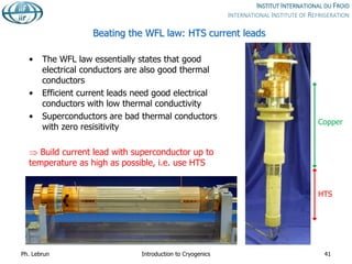
42. HTS vs. normal conducting current leads
Type
Resistive HTS (4 to 50 K)
Resistive (above)
Heat into LHe [W/kA] 1.1 0.1
Total exergy
consumption
[W/kA] 430 150
Electrical power
from grid
[W/kA] 1430 500
Ph. Lebrun Introduction to Cryogenics 42

43. Contents
• Introduction
• Cryogenic fluids
• Heat transfer & thermal insulation
• Thermal screening with cold vapour
• Refrigeration & liquefaction
• Cryogen storage
• Thermometry
Ph. Lebrun Introduction to Cryogenics 43

44. Basic thermodynamics of refrigeration
• First principle (Joule) 𝑄0 = 𝑄𝑖 + 𝑊
• Second principle (Clausius)
𝑄0
𝑇0
≥
𝑄𝑖
𝑇𝑖
• Hence 𝑊 ≥ 𝑇0
𝑄𝑖
𝑇𝑖
− 𝑄𝑖
Ph. Lebrun Introduction to Cryogenics 44
• This equation can be written in three different ways
𝑊 ≥ 𝑇0 ∆𝑆𝑖 − 𝑄𝑖 introducing entropy 𝑆 defined by ∆𝑆𝑖 =
𝑄𝑖
𝑇𝑖
𝑊 ≥ 𝑄𝑖
𝑇0
𝑇𝑖
− 1 where
𝑇0
𝑇𝑖
− 1 is called the Carnot factor
𝑊 ≥ ∆𝐸𝑖 introducing exergy 𝐸 defined by ∆𝐸𝑖 = 𝑄𝑖
𝑇0
𝑇𝑖
− 1
R
Qi
Q0
T0= 300 K
Ti
W : mechanical
work
(= for reversible process)

45. Minimum refrigeration work
• Consider the extraction of 1 W at liquid helium temperature 4.5 K, rejected at
room temperature 300 K
• The minimum refrigeration work is
𝑊𝑚𝑖𝑛 = 𝑄𝑖
𝑇0
𝑇𝑖
− 1 = 1
300
4.5
− 1 ≅ 65.7 W/W
• In practice, the most efficient helium refrigerators have an efficiency 𝜂 of
about 30% with respect to the Carnot limit
𝑊𝑟𝑒𝑎𝑙 =
𝑊𝑚𝑖𝑛
𝜂
=
65.7
0.3
≅ 220 W/W
Ph. Lebrun Introduction to Cryogenics 45

46. Refrigeration cycles
• Introducing the temperature-entropy diagram
– Consider the thermodynamic transform from A to B,
involving heat transfer ∆𝑄
– If it is reversible ∆𝑄 = 𝐴
𝐵
𝑇 𝑑𝑆
– ∆𝑄 is proportional to the area under the curve in
the temperature-entropy diagram
• To make a refrigeration cycle, one needs a
substance, the entropy of which depends on
some other physical variable than temperature,
e.g.
– Pressure of gas or vapor (compression/expansion)
– Magnetization of solid (magnetic refrigeration)
• Refrigeration cycle ABCD
– ∆𝑄1 heat absorbed at 𝑇1
– ∆𝑄2 heat rejected at 𝑇2
Ph. Lebrun Introduction to Cryogenics 46
A
B
T
S, entropy
Q
A B
T
S
C
D
T1
T2
Q1
Q2

47. T-S diagram for helium
H= 30 J/g
40
50
60
70
80
90
100
110
120
130
140
2
3
4
5
6
7
8
9
10
11
12
13
14
15
16
17
18
19
20
21
22
23
24
25
0 5000 10000 15000 20000 25000
Entropy [J/kg.K]
Temperature
[K]
P= 0.1 MPa
0.2
0.5
1
5
10 2
= 2 kg/m³
5
10
20
50
100
Ph. Lebrun 47
Introduction to Cryogenics
Red : liquid-vapour dome
Blue : isobars
Black : isochores
Green: isenthalps

48. A Carnot cycle is not feasible for helium liquefaction
• It would need a HP of 613 kbar!
• There exists no true isothermal
compressor
• There exists no true isentropic
compressor or expander
T
S
4.5 K
300 K
1.3 bar
613 kbar 82 kbar
3.89 J/g.K 8.07 J/g.K
Ph. Lebrun Introduction to Cryogenics 48

49. A real cycle needs internal heat exchange and para-isothermal compression
3.89 J/g.K 8.07 J/g.K
T
S
4.5 K
300 K
1.3 bar
20 bar
Practical compressors are adiabatic, need
aftercooling and if multistage, intercooling
Heat exchanger between
HP and LP streams
Ph. Lebrun Introduction to Cryogenics 49

50. Refrigerator Liquefier
4.5 K
S
Q1
T
4.2 J.g-1
.K-1
18.8 J.g-1
LOAD
Cold Box
LP
HP
Compressor
Q1
T1= 4.5 K
T0= 300 K
LOAD
Cold Box
LP
HP
Compressor
Q1
T1= 4.5 K
T0= 300 K
LHe
R
4.5 K
S
Q1
T
300 K
R
4.2
J.g-1
.K-1
23.1
J.g-1
.K-1
18.8 J.g-1
1543 J.g-1
isobar
(1.3 bar)
Ph. Lebrun Introduction to Cryogenics 50

51. Thermodynamic equivalence
between refrigeration and liquefaction
• What is the equivalent to 1 g helium liquefaction in terms of isothermal
refrigeration at liquid helium temperature 𝑇1 = 4.5 K ?
𝑊𝑙𝑖𝑞 = 𝑚𝑙𝑖𝑞(𝑇0 ∆𝑆 − 𝑄1 − 𝑅)
with 𝑇0 = 300 K
∆𝑆 = 27.3 J/g. K
𝑄1 = 18.8 J/g
𝑅 = 1543 J/g
hence 𝑊𝑙𝑖𝑞 = 6628 J
• Write that the same work is used to produce isothermal refrigeration at 4.5 K
𝑊𝑟𝑒𝑓 = 𝑄1
𝑇0
𝑇1
− 1 = 6628 J
hence 𝑄1 ≅ 100 J
• For refrigerators and liquefiers of the same efficiency
1 g/s liquefaction  100 W refrigeration at 4.5 K
Ph. Lebrun Introduction to Cryogenics 51

52. Measured refrigeration/liquefaction equivalence
12 kW @ 4.5 K helium refrigerators for LEP 2
Thermodynamic equivalence
Ph. Lebrun Introduction to Cryogenics 52

53. Elementary cooling processes on T-S diagram
P1
P2 (< P1)
T
S
A
B1
B2
B'2
B3
isobar
(heat exchanger) adiabatic (expansion engine)
isentropic
isenthalpic
(Joule-Thomson valve)
H
Ph. Lebrun Introduction to Cryogenics 53

54. Brazed aluminium plate heat exchanger
Ph. Lebrun Introduction to Cryogenics 54

55. Elementary cooling processes on T-S diagram
P1
P2 (< P1)
T
S
A
B1
B2
B'2
B3
isobar
(heat exchanger) adiabatic (expansion engine)
isentropic
isenthalpic
(Joule-Thomson valve)
H
Ph. Lebrun Introduction to Cryogenics 55

56. Cryogenic
turbo-expander
Ph. Lebrun Introduction to Cryogenics 56

57. Elementary cooling processes on T-S diagram
P1
P2 (< P1)
T
S
A
B1
B2
B'2
B3
isobar
(heat exchanger) adiabatic (expansion engine)
isentropic
isenthalpic
(Joule-Thomson valve)
H
Ph. Lebrun Introduction to Cryogenics 57

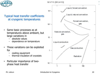
58. Joule-Thomson inversion temperatures
Cryogen
Maximum inversion
temperature [K]
Helium 43
Hydrogen 202
Neon 260
Air 603
Nitrogen 623
Oxygen 761
While air can be cooled down and liquefied by JT expansion from room temperature,
helium and hydrogen need precooling down to below inversion temperature by heat
exchange or work-extracting expansion (e.g. in turbines)
Ph. Lebrun Introduction to Cryogenics 58
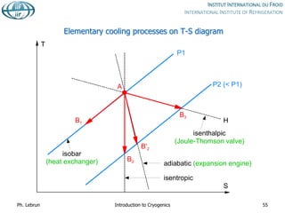
Isenthalps in T-S diagram can
have positive or negative slope,
i.e. isenthalpic expansion can
produce warming or cooling
 inversion temperature

59. Two-stage Claude cycle
Ph. Lebrun Introduction to Cryogenics 59

60. Claude-cycle helium refrigerators/liquefiers
Air Liquide & Linde
HELIAL SL HELIAL ML HELIAL LL
Max. Liquefaction capacity without LN2 25 L/h 70 L/h 145 L/h
Max. Liquefaction capacity with LN2 50 L/h 150 L/h 330 L/h
Compressor electrical motor 55 kW 132 kW 250 kW
Specific consumption for liquefaction w/o LN2 645 W/W 552 W/W 505 W/W
% Carnot 10% 12% 13%
Ph. Lebrun Introduction to Cryogenics 60

61. T5
4.5 K - 20 K loads
(magnets + leads + cavities)
T7
T1
T2
T3
T4
T8
T6
E1
E7
E3
E4
E6
E8
E9a
E9b
E10
E11
E12
E13
LN2
Precooler
20 K - 280 K loads
(LHC current leads)
50 K - 75 K loads
(LHC shields)
Adsorber
T1
T3
T7
T4
T8
T5
T6
201 K
75 K
49 K
32 K
20 K
13 K
10 K
9 K
4.4 K
0
.
1
M
P
a
0
.
4
M
P
a
1
.
9
M
P
a
0
.
3
M
P
a
T2
LHC shields
To LHC loads
from LHC loads
from LHC loads
Process cycle & T-S diagram of LHC
18 kW @ 4.5 K cryoplant
Ph. Lebrun 61
Introduction to Cryogenics

62. LHC 18 kW @ 4.5 K helium cryoplants
33 kW @ 50 K to 75 K
23 kW @ 4.6 K to 20 K
41 g/s liquefaction
4 MW compressor power
C.O.P. 220-230 W/W @ 4.5 K
Air Liquide
Linde
Ph. Lebrun Introduction to Cryogenics 62

63. ITER 25 kW @ 4.5 K helium refrigerator
Ph. Lebrun Introduction to Cryogenics 63

64. Oil-injected screw compressor
Ph. Lebrun Introduction to Cryogenics 64

65. Compressor station
of LHC 18 kW@ 4.5 K helium refrigerator
Ph. Lebrun Introduction to Cryogenics 65

66. Carnot, Stirling and Ericsson cycles
All «sloping» cycles need
internal heat exchange
For small machines, this
is done by regenerative,
rather than recuperative
heat exchangers
 alternating rather than
continuous operation
Ph. Lebrun Introduction to Cryogenics 66

67. Operation of a Gifford-
McMahon cryocooler
(Ericsson cycle)
Ph. Lebrun Introduction to Cryogenics 67

68. Two-stage Gifford-McMahon cryocooler
CRYOMECH PT407 & CP970 compressor
~ 0.7 W @ 4.2 K & 25 W @ 55 K
Ph. Lebrun Introduction to Cryogenics 68

69. Stirling and pulse-tube cryocoolers
Ph. Lebrun Introduction to Cryogenics 69

70. Mini pulse-tube cryocoolers
ESA MPTC development model – 1W @ 77K
CEA/SBT coaxial PTC– 6W @ 80K
Ph. Lebrun Introduction to Cryogenics 70

71. Contents
• Introduction
• Cryogenic fluids
• Heat transfer & thermal insulation
• Thermal screening with cold vapour
• Refrigeration & liquefaction
• Cryogen storage
• Thermometry
Ph. Lebrun Introduction to Cryogenics 71

72. Bulk helium storage solutions
11000 gallon liquid container
2 MPa gas tanks
20 MPa gas cylinders
Ph. Lebrun JUAS 2017 Intro to Cryogenics 72

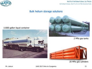
73. Specific cost of bulk He storage
Type
Pressure
[MPa]
Density
[kg/m3]
Dead volume
[%]
Cost
[CHF/kg He]
Gas Bag 0.1 0.16 0 300(1)
MP Vessel 2 3.18 5-25 220-450
HP Vessel 20 29.4 0.5 500(2)
Liquid 0.1 125 13 100-200(3)
(1): Purity non preserved
(2): Not including HP compressors
(3): Not including reliquefier
Ph. Lebrun JUAS 2017 Intro to Cryogenics 73

74. Contents
• Introduction
• Cryogenic fluids
• Heat transfer & thermal insulation
• Thermal screening with cold vapour
• Refrigeration & liquefaction
• Cryogen storage
• Thermometry
Ph. Lebrun Introduction to Cryogenics 74

75. 0,1 1 10 100 1000
He vapour pressure
He 3 gas thermometer
He 4 gas thermometer
Pt resistance thermometer
Temperature [K]
H2 Ne O2 Ar Hg H2O
Triple points
Definition of ITS90 in cryogenic range
Ph. Lebrun Introduction to Cryogenics 75
Primary thermometers

76. Primary fixed points of ITS90 in cryogenic range
Fixed point Temperature [K]
H2 triple point 13.8033
Ne triple point 24.5561
O2 triple point 54.3584
Ar triple point 83.8058
Hg triple point 234.3156
H2O triple point 273.16 (*)
(*) exact by definition
Ph. Lebrun Introduction to Cryogenics 76

77. From temperature sensor to practical thermometer
1cm
Ge
RhFe wire
RhFe thin film
Cernox
Carbon A-B
Carbon TVO
CBT
Ph. Lebrun Introduction to Cryogenics 77

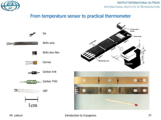
78. Practical temperature range
covered by cryogenic thermometers
1 10 100
Chromel-constantan
thermocouple
Au-Fe thermocouple
Pt resistance
Rh-Fe resistance
CLTS
Allen-Bradley carbon
resistance
Cernox
Ge resistance
Temperature [K]
Ph. Lebrun Introduction to Cryogenics 78

79. Some references
Books
• K. Mendelssohn, The quest for absolute zero, McGraw Hill (1966)
• R.B. Scott, Cryogenic engineering, Van Nostrand, Princeton (1959)
• G.G. Haselden, Cryogenic fundamentals, Academic Press, London (1971)
• R.A. Barron, Cryogenic systems, Oxford University Press, New York (1985)
• B.A. Hands, Cryogenic engineering, Academic Press, London (1986)
• S.W. van Sciver, Helium cryogenics, Plenum Press, New York (1986, 2nd edition 2012)
• K.D. Timmerhaus & T.M. Flynn, Cryogenic process engineering, Plenum Press, New
York (1989)
• J.G. Weisend (ed.), The handbook of cryogenic engineering, Taylor & Francis,
Philadelphia (1998)
• J.G. Weisend (ed.), Cryostat design: case studies, principles and engineering,
Springer, Switzerland (2016)
Ph. Lebrun Introduction to Cryogenics 79

80. Some references
Reports & Proceedings
• Ph. Lebrun, An introduction to cryogenics, CERN-AT-2007-01 (2007)
http://cdsweb.cern.ch/record/1012032?ln=en
• Proceedings of CAS School on Superconductivity and Cryogenics for Particle
Accelerators and Detectors, Erice (2002)
– U. Wagner, Refrigeration
– G. Vandoni, Heat transfer
– Ph. Lebrun, Design of a cryostat for superconducting accelerator magnet
– Ph. Lebrun & L. Tavian, The technology of superfluid helium
http://cdsweb.cern.ch/record/503603?ln=en
• Proceedings of CAS School on Superconductivity for Accelerators, Erice (2013)
– P. Duthil, Basic thermodynamics
– P. Duthil, Material properties at low temperatures
– A. Alekseev, Basics of low-temperature refrigeration
– B. Baudouy, Heat transfer and cooling techniques at low temperature
– V. Parma, Cryostat design
– Ph. Lebrun & L. Tavian, Cooling with superfluid helium
https://cds.cern.ch/record/1507630?ln=en
• Proceedings of ICEC, CEC/ICMC and IIR Cryogenics conferences
Ph. Lebrun Introduction to Cryogenics 80