shi_summer_2015

Topics in Exploring the Local Universe
through Density Maps of Various Celestial Objects
Tiger Shi
Advisor: Dr. James Annis
Research Completed During Summer 2015 at
Fermilab National Accelerator Laboratory
Batavia, Illinois
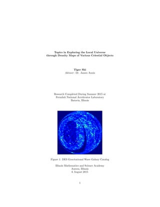
Figure 1: DES Gravitational Wave Galaxy Catalog
Illinois Mathematics and Science Academy
Aurora, Illinois
6 August 2015
1

topics in exploring the local universe through density maps of various celestial objects 1
Table of Contents:
1. Building Maps of the Galactic Halo:
I - Selecting RC Stars from Cas Jobs
II - Map Projections
III - Halo RC Stars Using Galaxia Foreground Subtrac-
tion:
i. Smoothing
ii. Reflections
IV - Halo RC Stars Using Trilegal Foreground Subtrac-
tion:
i. Reflections
V - Halo RC Stars Using DES Data with Trilegal and Galaxia
Foreground Subtraction
i. Reflections
2. Building Maps of z~1
3 Galaxy Distribution:
I - Literature
II - DES PhotoZ Catalog Maps
3. Conclusion

Building Maps of the Galactic Halo
Working with the SDSS and DES red clump star data, I try to map
out the large scale structure of the immediate local universe including
the our stellar streams, e.g. the Sagittarius Stream and the Orphan
Stream, as well as smaller high density dwarf galaxies. Utilizing the
Galaxia and Trilegal models, it was possible to complete some fore-
ground subtraction to bring out features hidden in the data gathered
in the two surveys.
Selecting RC Stars from Cas Jobs
Obtaining the SDSS Data required me to first search through the
papers of the two prior IMSA researchers, Arianna Osar and Anabel
Rivera, for SQL Queries that would allow me to retrieve only red
clump stars from the SDSS Skyserver data set through CasJobs. These
specific queries were taken from their papers in which they found out
the qualities unique to red clump stars and the specific regions of the
sky that they worked with.
Figure 1: SQL from left to right for
Osar's RC Stars and Rivera's Northern
RC Stars.
The reason red clump stars were chosen for mapping is due to two
main reasons. The first is that they are sparse and any high density
detections would allow us to be able actually visualize and notice.
Secondly, they have a very narrow magnitude range so that they are
easier to have they distances measured and be able to be distance
binned.

Map Making
Generating maps with the retrieved RC Star information requires
knowledge of applying the python module "matplotlib." The diffi-
culties in theory lies within deciding on the details of how the map
should be presented.
One such question lies in deciding between using Equatorial coor-
dinates or Galactic coordinates. The two different coordinate systems
are plotted below on star density maps of the Northern RC Stars.
50 100 150 200 250 300 350
Longitude
10
20
30
40
50
60
70
80
Latitude
Galactic l & b Map (indexed)
0
200
400
600
800
1000
1200
1400
1600
1800
50 100 150 200 250 300 350
ra
20
0
20
40
60
80
dec
ra & dec Map (indexed)
0
300
600
900
1200
1500
1800
2100
2400
2700
Figure 2: From left to right are star
density maps of the Northern RC Stars
Organized by l and b and the Northern
RC Stars Captured in Respect to ra and
dec.
Looking at the two maps, it can be seen that the same points plot-
ted in respect to two different references result in similar looking yet
wildly different plots. This is due to the scope of these two points of
view. Galactic longitude and latitude (l and b) is a system that uses the
Galactic equator as a frame of reference for angular distance. These
measurements use the sun as the center reference and the angles be-
ginning from at a line joining the sun and the Galactic Center. This
explains the high density area near (0,0) on the l and b plots which
is the Galactic Center along with (360,0) due to the cylindrical Plate
Carree projection. On the other hand, the Northern Galactic Pole is the
range between (0,90) and (360,90) due to the projection as well. Finally
as a result of this being a Northern Hemisphere Survey, the range of
−90 < b < 0 is not shown in this plot.
On the other hand, the RA vs DEC plots show a different view of
this map. Right ascension and declination are measurements of the
sky as it is projected onto an imaginary sphere above the Earth known
as the Celestial Sphere. These two measurements then measure the
angle an object is from the point of verneral equinox when the eclip-
tical and celestial equators intersect. They then follow in respect to
the celestial equator for the rest of the year. As a result the plots in

respect to these measurements are more relatable in that they are from
the reference point of a viewer on Earth. The center of this plot is the
Galactic Anticenter at about (180,45), while the much denser region at
around (270,0) and (90,0) is the Galactic Center.
Splitting up the data is yet another decision to make when cus-
tomizing maps for others to view. However, this is a much more
case-based issue in that the way that one wants to present a plot may
cause indexing to vary depending on the data sets and desired results.
There are various reasons for deciding what data to reject adn cutting.
Often times it was found that the data also contained mislead-
ing points that were resulted from equipment errors or false objects.
These were taken out via indexing. This process involved creating a
histogram of the magnitude of 'r' before making the hexagonal bin-
ning plot due to its higher tractability. This will allow for the false
datum to be easily identiﬁable and to have a range index set around
the useful data points. The index used for this data is 15 < r < 16, elim-
inating all stars outside these bounds as can be seen in the following
image.
8 9 10 11 12 13 14 15 16 17
r Magnitude
0
20000
40000
60000
80000
100000
NumberofStars
Indexed vs Unindexed
Figure 3: Visualizing indexing with stars
from Anabel's data. The blue histogram
is the unindexed data, while the green
is the data after being indexed into
15 < r < 16
The final important decision that is needed to be made is in
the projection of the map. The two I used during this summer are
the Plate Carree and the Lambertian Equal Area Projections. Both
have their advantages and faults but the Lambertian Equal Area (EA)

Projection was a much more useful projection for the purposes of my
research.
The Lambertian EA Projection is a type of planar projection that
aims in preserving acurate areas per pixel as a primary goal. It looks
to accommodate Equatorial, Polar, and Oblique properties in between
the original and the projection. The only distortions that seem to
take place occur radially outwards. In this project, this projection
will be used mainly for mapping Galactic longitude l and latitude b.
However, Figure (4) will demonstrate this projection style with right
ascension and declination.
6 4 2 0 2 4 6
6
4
2
0
2
4
6
Lambertian EA Projection of Full Sky Galaxy Catalogue
0
40
80
120
160
200
240
280
Figure 4: Lambertian Equal Area
Projection of the Gravitational Wave
galaxy catalog using the ra and dec
rather than l and b. Indexing was used
in respect to the i-Band Magnitude
from 14 to 17 since the entirety of major
activity can be found within that range.
Generating this kind of projection requires using an equation
(Equation (1)) found in J.A. Steeres' An Introduction to the Study of
Map Projections and some work with the polar coordinate system.1 The 1
Steers, J.: 1962, An Introduction to the
Study of Map Projections, University of
London Press LTD
process moves through manipulation of the equation and converting
it to respond to ra & dec and l & b. Key items to keep in mind for this
is to ensure that the degrees to be converted into radians through the
equations and that the image must be able to ﬁt on a 8.5”x11” page
with at least 1 inch margins. (R is the radius of the physical resulting
projection and in this case will be set as 3.25 inches chosen in respect
to the printer paper.) The result can be seen in Equation (2) and (3)
which have the x and y coordinates, respectively, that would yield a
Lambertian Equal Area Projection. These can then be directly inserted
into the Python plotting code to allow for easy plotting.

(ra, dec) → (l, b)
θ = ra
R = 3.25inches
r =
√
2R
√
1 − sin(dec) (1)
x = r × cos(θ) = r × cos(ra)
y = r × sin(θ) = r × sin(ra)
x = R × cos(ra)
√
2(1 − sin(dec))
y = R × sin(ra)
√
2(1 − sin(dec))
x = 3.25 × cos(
ra × π
180
)
√
2(1 − sin(
dec × π
180
)) (2)
y = 3.25 × sin(
ra × π
180
)
√
2(1 − sin(
dec × π
180
)) (3)
To fully realize what a Lambertian l and b Projection would look
like, I had applied the same technique on the data sets retrieved from
the SQL queries found in Anabel Rivera's paper and Arianna Osar's
paper entered onto CASJOBS, both of which yielded data that con-
tained Galactic Longitude and Latitude. The plots are shown in Fig-
ures (5) and (6) respectively. They both seem to yield agreable results
since they contain a similar region of space. However since Arianna's
data covered some parts of the Southern Hemisphere along with the
common Northern Hemisphere and the Lambertian Azimuthal Equal
Area Projection distorts radially past the Equator, the projection of her
data appeared much more distorted than Anabel's. The edges seem to
suffer from a fish-eye effect seemingly being stretched out in a ring as
compared to the projection derived from Anabel's data which seems
to sensibly preserve area and a believable shape.

6 4 2 0 2 4
2
0
2
4
6
Lambertian EA Projection of l and b of Ari's RC Stars
0
1500
3000
4500
6000
7500
9000
10500
12000
4 3 2 1 0 1 2 3 4
3
2
1
0
1
2
3
4
Lambert Equal Area of North Cap
0
250
500
750
1000
1250
1500
1750
2000
2250
The ﬁrst plot was formed using l and b from the query from Ari-
anna's paper. Covering both the Northern Hemisphere and part of
the Southern Hemisphere, the edges of this projection seem to be dis-
torted and stretched out. The second plot, however, was formed using
l and b from using the query from Anabel's paper. Contrary to Ari-
anna's data, this data only covered the Northern Hemispher and not
passing the Equator. This causes there to be no similar distortion and
a clearer idea at what the plot is attempting to communicate.

Mapping Halo RC Stars using Galaxia Foreground Sub-
traction
Applying the map making skills, map projections can now be
used for scientific inquiries rather than just as practice to make more
maps. Using the SDSS red clump data by itself would not be able to
tell much about the local universe in that it is so cluttered with the
structures around us such as the Milky Way Galaxy's bulge and disk.
To clean up the view, a filter must be applied to weed out unwanted
values. This would be the job for models such as Galaxia. When the
red clump selection of Galaxia is subtracted from the SDSS Data, the
result would be a clearer view of the streams and structures surround-
ing us.
In order to work with the cellestial bodies and detect voids and
clumps, it is required to have a map that is accurate enough and cov-
ers enough area so that one would get a decent understanding of area
that is being worked with. To do this, we found data of the Sloan Dig-
ital Sky Survey that covered the Northern and Southern hemisphere
from 5-70 kiloparsecs (kpc) away. This data was then split into eight
different distance bins, i.e., 5, 10, 20, 30, 40, 50, 60, and 70 kpc. The
distances were found via the distance modulus:
µ = m − M (4)
d = 10
µ
5 +1
(5)
In the Equation (4), "µ" is called the distance modulus and is the
difference between "m," the apparent magnitude, and "M," the abso-
lute magnitude. With the value of "µ" found, Equation (5) can be used
to solve for "d," the distance the object is away from us in parsecs (pc).
The Distance bins for the North and the South Hemispheres smoothed
at 7σcan be found in Appendix A.
Smoothing
Using this as the determining factor, it allowed us then to split the
massive collection of data into sets of data specific to a certain dis-
tance away. However, maps made directly from the points collected
in these distance bins are not dense enough for most humans to be
able to interpret the existance of an over or underdensity. Luckily,
the problem can be solved by Gaussian smoothing. (I chose to use a
Guassian smoothing of 7σdue to personal preferences.) This can be
demonstrated in the following figures.

0 500 1000 1500
0
500
1000
1500
SDSS North at 30kiloparsecs at sigma=0
12
8
4
0
4
8
12
0 500 1000 1500
0
500
1000
1500
3.2
2.4
1.6
0.8
0.0
0.8
1.6
2.4
3.2
Figure 5: Before and After of 7σGaus-
sian Smoothing on 30 kpc North RC
Stars.
0 500 1000 1500
0
500
1000
1500
SDSS South at 30kiloparsecs at sigma=0
5.0
2.5
0.0
2.5
5.0
7.5
10.0
12.5
15.0
17.5
20.0
0 500 1000 1500
0
500
1000
1500
5.0
2.5
0.0
2.5
5.0
7.5
10.0
12.5
15.0
17.5
20.0
Figure 6: Before and After of 7σGaus-
sian Smoothing on 30 kpc South RC
Stars.

Results and Explanations
To understand the implications of the data, we must first
understand the plots and what they are saying. In both the North and
the South maps, the irregularly shaped structure with tendrils and
dots coming off of it are the SDSS RC Stars. The white circle centered
in the middle of the map is the area in which the RC star selection of
Galaxia model resides. The dark region beyond the circle is where
there is data but no model, while the area that is pure white is where
there exists a model but no data. what is left is the fuzzy gray area,
which is the residual that resulted from the Galaxia model being
subtracted from the SDSS data.
Mapping Halo RC Stars using Trilegal Foreground Sub-
traction
The Galaxia residuals seemed to be rather effective in bringing
out features in the Northern Hemisphere SDSS RC Stars. Through
most of the distance slices, the Sagittarius Stream and Virgo Overden-
sity could be seen. However, the story is very different for the pieces
in the Southern Hemisphere. For every single distance slice, the pic-
ture was empty it was too smooth overall with a strange saturation in
the top right corner which could have either been a fault in the fore-
ground subtraction or the Monoceros Ring. To make sure that this was
not an error, a new foreground subtraction model was chosen. This
new model was called Trilegal which stood for the TRIdimensional
modeL of thE GALaxy.
Figure 7: SDSS South RC Star Data
Residual by Trilegal Model at 40 and 60
kpc respectively.

Results and Explanations
Although there was high hopes for the new residuals to reveal more
structure, the Trilegal model was, unfortunately, unable to ﬁt with the
SDSS Data. This version of Trilegal that I found was designed to be
used for the DES Data so it does not cover areas with DEC > 0 or b > 0.
As seen in Figure 8.
300 350 400 450
ra
80
60
40
20
0
dec
Trilegal Model: Plate Carree
0
4000
8000
12000
16000
20000
24000
28000
32000
50 100 150 200 250 300 350
Galactic Longitude
80
60
40
20
0
GalacticLatitude
0
8000
16000
24000
32000
40000
48000
56000
64000
Figure 8: Star Density per Pixel map
of the Trilegal Model mapped with
RA/DEC and l/b respectively.
Due to these limitations, the SDSS Data and Trilegal model could
only yield a thin slice of usable residual with the rest of the model
and data not overlapping each other. However, these slices did show
something interesting in that there seems to be a surprisingly darker
region where the Sagittarius Stream should cover in the Southern
Hemisphere, but cannot be conﬁrmed if it truly exists due to the size
of the residual showing it.
Mapping Halo RC Stars using DES RC Data with Tri-
legal and Galaxia Foreground Subtraction
To strengthen the claim that there is large scale structure in the
Southern Celestial Hemisphere, the DES data was enlisted to help
uncover more of the area covered by the Trilegal model. The maps
of the DES Galaxies plotted over the Galaxia model and the Trilegal
Model can be seen in Appendix B.
When a foreground subtraction using the Trilegal model on the
DES data was done at a 30 kiloparsec distance bin, the same struc-
ture as seen in the SDSS data of the same distance bin in the overlap
between the two showed up again. This bolsters the claim that large
scale structure, possibly the Sagittarius Stream, may exist in the South-
ern Hemisphere.

Building Maps of z~1
3 Galaxy Dis-
tribution
Planck was satellite that functioned as a space observatory between
2009 and 2013 for the European Space Agency. Its goal was to map
out the Cosmic Microwave Background radiation which is ancient
infra-red and thermal radiation that is thought to be residual to the
origin of the universe. However while mapping this radiation, an
anomaly came into view. There seemed to be a significant underden-
sity at l=207.8°and b=-56.3°. This is an improbable event as such an
underdensity shouldn't exist in a homogeneously random universe.
The CMB Cold Spot then brought about many projects to study its
existence and origins.
Literature
To gain an understanding on the extent of the research on the Cosmic
Microwave Background Cold Spot detected by the Planck satellite has
reached. Three readings were assigned:
• Detection of a supervoid aligned with the cold spot of the cosmic
microwave background2 2
Szapudi, I., Kovács, A., Granett, B. R.,
Frei, Z., Silk, J., Burgett, W., Cole, S.,
Draper, P. W., Farrow, D. J., Kaiser, N.,
Magnier, E. A., Metcalfe, N., Morgan,
J. S., Price, P., Tonry, J., and Wainscoat,
R.: 2015, Monthly Notices of the RAS 450,
288
• A redshift survey towards the CMB Cold Spot3
3
Bremer, M. N., Silk, J., Davies, L. J. M.,
and Lehnert, M. D.: 2010, Monthly No-
tices of the RAS 404, L69
• Galaxy counts on the CMB Cold Spot4
4
Granett, B. R., Szapudi, I., and
Neyrinck, M. C.: 2010, Astrophysi-
cal Journal 714, 825
Each of these studies used a different method of analyzing the Cold
Spot and the cause of such an anomaly. With the discovery of this
Cold Spot being so young, many hypotheses have been made in order
to understand the roots and reasons for this hole in the CMB.
Szapudi's study was rather straightforward. His team had used the
WISE-2MASS infrared galaxy catalogue along with the Pan-STARRS1
galaxies to look for a supervoid in the direction and location of the
detected Cold Spot. They looked through different ranges of redshifts
between two angular radii, i.e., 5°and 15°. Being that the team was
searching for a void in the Cold Spot, they evidence that suggested
low galaxy densities with high significance of detection. All in all,
Szapudi's team claimed to have gathered enough evidence to prove
the existance of a supervoid existing as the cause for the Cold Spot in
the CMB.5 5
Szapudi, I., Kovács, A., Granett, B. R.,
Frei, Z., Silk, J., Burgett, W., Cole, S.,
Draper, P. W., Farrow, D. J., Kaiser, N.,
Magnier, E. A., Metcalfe, N., Morgan,
J. S., Price, P., Tonry, J., and Wainscoat,
R.: 2015, Monthly Notices of the RAS 450,
288
Bremer's study, however, had differing results. Bremer and his team
used the VIMOS Spectrograph on the Very Large Telescope (VLT) at

the Cold Spot. Contrary to what Szapudi's team had found, Bremer
found that the Integrated Sachs-Wolfe effect due to a supervoid at
reshift between 0.5 and 1 is not a viable candidate for the production
of a Cold Spot in the Cosmic Microwave Background.6 Bremer's team 6
tices of the RAS 404, L69
deduced that there are other reasons that may cause the Cold Spot to
come into existance such as:
• The void exists in a redshift lower than tested here
• "New Physics" is at play here
• New approaches to data analysis may be needed7 7
tices of the RAS 404, L69Although Bremer seemed rather confident in his conclusions, upon
closer inspection of his data it can be seen that there are faults in his
work. The biggest issue is that his team had selected an extremely
tiny portion of the Cold Spot to analyze. Even with a small amount
of smoothing, his test area was barely 10% of the total Cold Spot area.
This made his analysis of the entire area to seem rather trivial with the
amount of area he had covered.
Granett and his team seemed to be split between the two opinions.
They used the MegaCam on the Canada-France-Hawai'i Telescope
and current galaxy counts to analyze much more expanded regions
of the Cold Spot when compared to Bremer's survey area. From
Granett's results, there is much evidence to suggest a possibility that
a supervoid is causing the Cold Spot, with a comfirmed (to 2MASS)
underdensity at low redshifts, 0.1 < z < 0.3, in the examined areas.
Contrary to Bremer, Granett does acknowledge that "due to the lim-
ited sky coverage of our [the] survey, we [Granett's team] cannot draw
a definite conclusion regarding the existance of a coherent supervoid
structure."8 8
Granett, B. R., Szapudi, I., and
Neyrinck, M. C.: 2010, Astrophysi-
DES Photo Z Catalog Maps
To locate the void, I had to first retrieve the DES Catalogs for Year
1 Annual Release 1 (Y1A1) and Year 2 Quick Release 1 (Y2Q1). Then
from these data sets I had to filter out everything that is not a galaxy
and map out the galaxies in a hexbin galaxy per pixel density map.
Four seperate redshift bins were established being 0.1 to 0.2, 0.2 to 0.3,
0.3 to 0.4, and 0.4 to 0.5, each representing a different time of origin
for the galaxies. The finished maps of the first set of specifications are
shown below.

2 1 0 1 2 3
3
2
1
0
1
2
DES South PhotoZ 0.1 to 0.2
0
800
1600
2400
3200
4000
4800
5600
6400
2 1 0 1 2 3
3
2
1
0
1
2
0
400
800
1200
1600
2000
2400
2800
2 1 0 1 2 3
3
2
1
0
1
2
0
400
800
1200
1600
2000
2400
2800
3200
3600
2 1 0 1 2 3
3
2
1
0
1
2
0
500
1000
1500
2000
2500
3000
3500
4000
4500
Figure 9: Galaxy Density maps of the
DES data from Y1A1 and Y2Q1 for
Redshift bins with i-Band Magnitude
less than 20.
As you can see in most of the maps from this first mapping, the
two data sets, Y1A1 and Y2Q1, did not match too well. The Y1A1 data
is the section that is dark blue in the 0.1 to 0.2 redshift map and the
Y2Q1 data is the light blue area. As we move through the redshift
cuts, the two sections seem to change in their densities. In the 0.1 to
0.2 cut, Y1A1 has a much lower density than the Y2Q1. In the 0.2 to
0.3, they seem to fit better. But in both the 0.3 to 0.4 cut and the 0.4 to
0.5 cut, the Y1A1 density has a significant overdensity when compared
to the Y2Q1 density. We know that this could not be a real structure in
the universe, because we know that the is more or less homogeneous
and that the density differences follow the edges of the surveys. This
led us to suspect something faulty with the data itself. To understand
what may be causing these problems, I made a histogram (Figure
10) of the photometric redshifts of both surveys in the range of the
redshifts used.

Figure 10: Photometric Redshift bins
displaying Y1A1 in Blue and Y2Q1 in
Green
As comﬁrmed by the histogram, there seems to have been a rather
signiﬁcant error in the Y2Q1 data in that it has an unusual pile-up
of Galaxies at a photometric redshift near 0.1. This is unusual since
typically galaxy counts tend to increase with increasing redshifts as
the data for Y1A1 does.
To correct the issues here, we created a few extra cuts in the data
which helped eliminate unwanted data points with faulty photometric
redshifts as marked by a MULT_NITER_MODEL that equal to 0 or a
SPREAD_MODEL_I that is less than 0.005. In doing so, the maps in
Figure 11 were created.

2 1 0 1 2 3
3
2
1
0
1
2
DES PhotoZ 0.1 to 0.2
0
200
400
600
800
1000
1200
1400
1600
2 1 0 1 2 3
3
2
1
0
1
2
0
100
200
300
400
500
600
700
800
900
2 1 0 1 2 3
3
2
1
0
1
2
0
150
300
450
600
750
900
1050
1200
2 1 0 1 2 3
3
2
1
0
1
2
0
80
160
240
320
400
480
560
640
Figure 11: Galaxy Density maps of
the DES data from Y1A1 and Y2Q1
for Redshift bins of 0.1 to 0.2, 0.2 to
0.3, 0.3 to 0.4, and 0.4 to 0.5 with
i-Band Magnitude less than 20 af-
ter cutting away faulty redshifts
with MULTN ITERMODEL > 0 and
SPREADMODELI > 0.005.
With the new cuts on the two DES survey data, there seems to be
a general improvement of over density homogeneity. However, there
can still be improvements done. Even though overall the maps seem
more even, both the 0.1 to 0.2 and the 0.2 to 0.3 cuts seem to have
an overdensity in Y1A1 now. Also the Y1A1 data of the 0.4 to 0.5 cut
seems to be a bit too low than what we want from it.
Conclusion
In building maps of the Galactic Halo using redclump star residuals,
challenges were faced in the process. Although the Northern Hemi-
sphere of the SDSS data ﬁt well with the Galaxia model in creating a
decypherable residual map, the Southern Hemisphere did not result
in such a success. As an attempt to solve the problem, the Trilegal
model was used for foreground subtraction instead of the Galaxia
model. This only resulted in barely any overlap between the SDSS red
clump data and the Trilegal model allowing for a very thin window of
residual. However, in the small sliver of residual from the map,there

is a hint in that there may be large scale structure that could not be
clearly seen in that Hemisphere.
To bolster that idea, the DES data for redclump stars was recruited
for foreground subtraction by both the Galaxia and the Trilegal mod-
els. The resulting maps of these residuals showed strong evidence
that would suggest that the previously acknowledged structure may
actually be the southern portion of the Sagittarius Stream.
In understanding the nature of the Planck CMB Cold Spot, galaxy
distribution maps of the Dark Energy Survey data at Photometric Red-
shift ~1
3
had to be made. These maps used two different releases of the
DES data being Y1A1 and Y2Q1 at 4 different redshift ranges between
0.1 and 0.5. However due to certain reasons, the two releases did not
have similar densities at their respective redshifts which resulted in
maps where the density sharply increased or decreased between re-
lease data.
In order to fix this, an attempt was made to eliminate data points
with faulty redshifts which was marked with certain cuts on the
MULT_NITER_MODEL and the SPREAD_MODEL_I components
of the DES data. The results seem to be a slight improvement but can
be further increased in homogeneity overall.

Appendices
Appendix A. Northern and Southern Hemisphere Plots of SDSS
Data from 5 to 70 kpc away
0 500 1000 1500
0
500
1000
1500
6.0
4.5
3.0
1.5
0.0
1.5
3.0
4.5
0 500 1000 1500
0
500
1000
1500
5.0
2.5
0.0
2.5
5.0
7.5
10.0
12.5
15.0
17.5
20.0
Figure 12: 0.5 kiloparsec bin
0 500 1000 1500
0
500
1000
1500
1
0
1
2
3
4
5
6
7
0 500 1000 1500
0
500
1000
1500
5.0
2.5
0.0
2.5
5.0
7.5
10.0
12.5
15.0
17.5
20.0
Figure 13: 10 kiloparsec bin

0 500 1000 1500
0
500
1000
1500
2
1
0
1
2
3
4
5
0 500 1000 1500
0
500
1000
1500
5.0
2.5
0.0
2.5
5.0
7.5
10.0
12.5
15.0
17.5
20.0
0 500 1000 1500
0
500
1000
1500
3.2
2.4
1.6
0.8
0.0
0.8
1.6
2.4
3.2
0 500 1000 1500
0
500
1000
1500
5.0
2.5
0.0
2.5
5.0
7.5
10.0
12.5
15.0
17.5
20.0

0 500 1000 1500
0
500
1000
1500
4.0
3.2
2.4
1.6
0.8
0.0
0.8
1.6
2.4
0 500 1000 1500
0
500
1000
1500
5.0
2.5
0.0
2.5
5.0
7.5
10.0
12.5
15.0
17.5
20.0
0 500 1000 1500
0
500
1000
1500
2.5
2.0
1.5
1.0
0.5
0.0
0.5
1.0
0 500 1000 1500
0
500
1000
1500
5.0
2.5
0.0
2.5
5.0
7.5
10.0
12.5
15.0
17.5
20.0

0 500 1000 1500
0
500
1000
1500
3.0
2.4
1.8
1.2
0.6
0.0
0.6
1.2
1.8
0 500 1000 1500
0
500
1000
1500
5
4
3
2
1
0
1
2
3
4
0 500 1000 1500
0
500
1000
1500
3.0
2.4
1.8
1.2
0.6
0.0
0.6
1.2
1.8
0 500 1000 1500
0
500
1000
1500
5.0
4.5
4.0
3.5
3.0
2.5
2.0
1.5
1.0
0.5
0.0

Appendix B. DES Data with Foreground Subtraction by Galaxia
and Trilegal at Various Distance Bins
Figure 20: DES Data residuals by
Galaxia Foreground Subtraction for 30,
40, and 50 kpc distance bins.

Figure 21: DES Data residuals by Trile-
gal Foreground Subtraction for 30, 40,
and 50 kpc distance bins.References
Bremer, M. N., Silk, J., Davies, L. J. M., and Lehnert, M. D.: 2010,
Monthly Notices of the RAS 404, L69
Granett, B. R., Szapudi, I., and Neyrinck, M. C.: 2010, Astrophysi-
Steers, J.: 1962, An Introduction to the Study of Map Projections, Univer-
sity of London Press LTD
Szapudi, I., Kovács, A., Granett, B. R., Frei, Z., Silk, J., Burgett, W.,
Cole, S., Draper, P. W., Farrow, D. J., Kaiser, N., Magnier, E. A., Met-
calfe, N., Morgan, J. S., Price, P., Tonry, J., and Wainscoat, R.: 2015,
Monthly Notices of the RAS 450, 288

shi_summer_2015

Recommended

Recommended

More Related Content

What's hot

What's hot (19)

Viewers also liked

Viewers also liked (11)

Similar to shi_summer_2015

Similar to shi_summer_2015 (20)

shi_summer_2015