1. Analysis of Metabolites Through Reciprocally
Regulated Pathways
Martin Kinisu, Thomas Glucksman
March 19, 2015
Abstract
The following presents a model that mathematically simulates the flux through
reciprocally regulated pathways common in eukaryotic biochemistry. Utilizing differ-
ential equations and their solutions, we were able to construct a model that displays the
changes in concentrations of glucose and glycogen. The mechanisms of interest were the
linked pathways of Glycolysis/Gluconeogenesis, and Glycogen synthesis and Glycogen
breakdown. The model accurately demonstrates the decrease and interchange of these
two species over time.
1 Introduction
The consumption of environmental nutrients and their conversion to readily usable energy
equivalents is a process shared by all living organisms. Humans utilize a broad diet to supply
themselves with the building blocks and energy that are necessary for life. In biochemistry,
glucose is considered the entry point of energy into the body. Whether obtained directly
from our diet in the form of carbohydrates and simple sugars, or indirectly in other forms
such as protein or fats, a persons blood glucose concentration is a clear indication of their
energy state.
After a meal the concentration of glucose in the bloodstream elevates. Utilization of the
energy stored in glucose comes from the biochemical breakdown of the molecule. Glycolysis
is the pathway in most eukaryotes that performs this task. Starting with glucose, enzymes
and their cofactors work to break the molecule down into direct precursors for adenosine
triphosphate (ATP) which is essentially a stored form of the thermodynamic energy re-
quired to drive otherwise unfavorable or slow reactions in the body that are crucial for life.
Glycolysis is therefore the pathway that dominates during times of high energy requirement
e.g. exercise, growth, and stress. During periods of low energy requirement the body works
to store glucose for later use. This process occurs in two steps. First is the regeneration
of glucose from metabolites further downstream in the glycolytic pathways, and second is
the final storage of glucose in an efficient form. The regeneration of glucose is carried out
via a process called Gluconeogenesis. This process uses ATP to condense metabolites in
the glycolytic pathway into glucose. The glucose is then enzymatically added to a molecule
called glycogen, which is a large, branched polymer with glucose monomeric units. The
1

2. addition of glucose units to glycogen is termed Glycogen synthesis. In times of increasing
energy demand Glycogen is catabolized in its breakdown process. This yields free glucose
with can then enters Glycolysis and generate readily usable ATP.
These two pairs of breakdown and synthesis pathways are reciprocally regulated. This
essentially means that only one process in each pair can be on at any given time. When
glycolysis is active, gluconeogenesis is inhibited and vice versa. The same is also true for the
breakdown and synthesis of glycogen. If two of a pair were to be on at the same time, this
would constitute a futile cycle in which no net energy is being used or produced.
2 Assumptions
• Breakdown and synthesis pathways are never on at the same time
• Breakdown is the exact opposite of synthesis i.e. the negative of synthesis
• Energy demand is proportional to current glucose concentration
• Change in glucose is negatively affected by glycogen concentration, positively influ-
enced by energy input, and negatively influenced by energy demand
• Change in glycogen is proportional the current glucose concentration.
3 Model
As previously discussed we have established that the rate of glucose synthesis versus the
rate of glycogen synthesis are reciprocally related, so in order to represent this relationship
we must derive a model in which the rate of glucose synthesis is dependent on the rate of
glycogen synthesis and vice versa. So from there we need at least two time-dependent rates,
say dx
dt
and dy
dt
, where dx
dt
is dependent on dy
dt
.
Once we have established these dependencies we can denote each pathway with the
following equations:
dx1
dt
= −αy1(t) + n − E
dx2
dt
= −dx1
dt
(1)
dy1
dt
= βx1(t)
dy2
dt
= −dy1
dt
(2)
Each of these coupled systems correspond to glycolysis and gluconeogenesis. The reason
each of these equations exists as a coupled system of four equations is simply to indicate
that there also reverse processes denoted by the negative of the original forward pathway.
Without loss of generality, we will only be focusing on the forward direction. Beginning with
equation (1):
dx1
dt
= −αy1(t) + n − E
2

3. The constant α represents the enzymatic efficiency of gluconeogenesis, which determines
the rate at which metabolic intermediates further downstream in the glycolytic pathway
are being converted to back glucose. The reason this exists as a negative dependence is to
illustrate that this is a rate at which glucose is expended. Since we do not know exactly
the rate at which glucose is synthesized, we can at least derive an expression based on the
negative of the process that consumes it.
Additionally we see that equation (1) depends negatively on y1(t) and our energy demand
function E while having a positive dependence on another constant n which corresponds to
the initial energy intake, such as the amount of glucose taken in from a typical meal. Our
function E then corresponds to:
E = µx1(t) (3)
Where µ is a positive constant that represents the intensity of the energy requirement.
Higher values of µ correspond to a more extreme energy demand. The function of glucose
at a time t is denoted by x1(t).
Glycogen synthesis is modeled by the equation (2):
dy1
dt
= βx1(t)
Where β is the enzymatic efficiency of Glycogen synthesis, similar to α in equation (1).
Because the synthesis of glycogen is only dependent on the amount of glucose being created,
our equation is only dependent on x1(t).
4 Verification
To verify this model we will first examine the stability points equations (1) and (2) by solving
the following system:
dx1
dt
= −αy1(t) + n − E = 0
dy1
dt
= βx1(t) = 0
Solving for x1(t) we see that the only possible solution is x1(t) = 0. Equation (1) then
becomes:
dx1
dt
= −αy1(t) + n − µx1(t)
= −αy1(t) + n = 0
Solving for y1(t) we then get:
x1(t) = 0
y1(t) = n
α
Now that we have (x0, y0) = (0, n
α
) we can utilize a stability matrix:
d
dt
δx
δy
=
fx(x0, y0) fy(x0, y0)
gx(x0, y0) gx(x0, y0)
δx
δy
3

4. to analyze the behavior of the solution in order to verify the validity of our model when we
solve equations (1) and (2). Note that here f(x, y) = dx1
dt
and g(x, y) = dy1
dt
.
Then we have
fx(x0, y0) fy(x0, y0)
gx(x0, y0) gx(x0, y0)
=
−µ −α
β 0
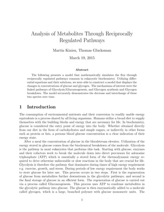
Next we analyze the sign of the determinant (∆) and trace (τ)of this matrix:
∆ = (−µ)(0) − (−α)(β) = αβ
τ = −µ + 0 = −µ
Figure 1: Dimensionless Cartesian phase-plane representing the range of trace (τ) and de-
terminant (∆) values possible, and the regions of qualitative behavior of linear systems.[1]
Finally we analyze the phase-plane pictured above to determined the stability of the
solution to our system based on the coordinate location of the trance and determinant of the
stability matrix. Since we have a positive determinant and negative trace (∆ > 0, τ < 0),
our point lies in the 4th quadrant, corresponding to a stable point.
From this analysis alone we cannot specify if our point classifies as a stable focus or stable
node, but for our purposes will will assume that the distinction will have little effect on our
overall result.
4

5. Figure 2:
Figure 3:
Now moving on to the actual solution, we utilized MATLAB’s built-in ode45 function to
solve a system of linear first-order differential equations to produce the above results.
The concentrations of both glucose and glycogen rise and fall in correspondence with each
other, and show a trend toward zero, where each solution eventually converges as indicated
by our stability analysis. Additionally, we notice the effects of varying our energy demand
constants.
We would expect that with an increased energy demand, our solution would converge
more quickly due to the fact that more resources need to be converted at any given time,
and the resources are also being depleted.
5

6. Figure 4:
Figure 5:
We also notice that increasing the enzymatic efficiency increases the frequency or rate
of oscillation between glucose and glycogen, which corresponds to the speed at which both
substances are converted. Figure 4 also shows the decrease in convergence when our energy
demand is low versus the sharp increase in convergence when it is high.
6

7. 5 Discussion
From these results we can conclude that overall the model was a success. Our convergence
condition follows in accordance with how the body consumes glucose, eventually depleting
this resource over time. The varying effects of our constants also follow in accordance with
our model, showing that altering the enzymatic efficiency or energy demand does have a
significant effect on the rate of change in glucose and glycogen concentrations.
Although our model is sufficient for showing the behavior of glucose and glycogen over
time, it assumes that there is only one initial intake of energy. Assuming that no glucose in
the body means death, this model only indicates that the person has eaten once and died
of starvation. Humans consume food on a daily basis, or at least they should in order to
maintain a healthy state, so while accurate, this model is not entirely realistic.
Figure 6: X1(t) = msin(t)sin(nπt), Y1(t) = mαsin(t)cos(nπt)
Ideally, we would want our solution to resemble something close to Figure 6, which shows
varying amplitudes that correspond to the intake as well as consumption of glucose, which
also converge to zero at some point.
Unfortunately, due to the limitations of modeling these pathways as a set first-order
ODEs, it does not seem possible to achieve a solution that exactly resembles Figure 6.
However, by adjusting the rate of energy demand to have an oscillating factor, we can derive
a model that approximates the desired behavior.
7

8. Figure 7:
By changing our energy demand function from E = µx1(t) to E = 0.05t(sin(nt))x1(t)
we arrive at a slightly irregular oscillatory behavior that follows our convergence result.
Although time in this case is not scaled properly, we can see that it is possible to somewhat
imitate the act of food consumption by adding an oscillating factor to our variables, and it
may be possible to model eating over a finite period of time. However, we believe that this
may require the use of second-order ODE’s or higher, which could possible be applied to this
specific pathway but would require a more in-depth study.
References
[1] Edward O. Keith A Matrix Model of Fasting Metabolism in Northern Elephant Seal Pups
2012.
8