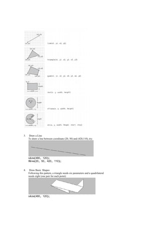
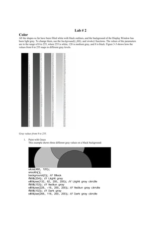
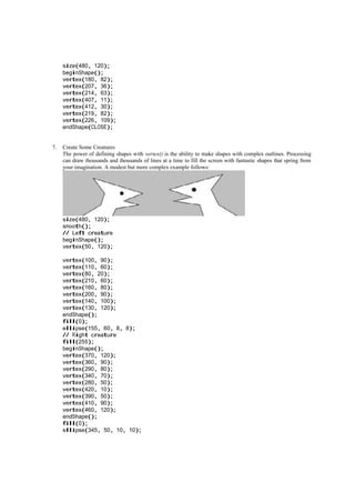
2. Lab # 1
Drawing in Processing
At first, drawing on a computer screen is like working on graph paper. It starts as a careful technical procedure, but
as new concepts are introduced, drawing simple shapes with software expands into animation and interaction.
Before we make this jump, we need to start at the beginning.
A computer screen is a grid of light elements called pixels. Each pixel has a position within the grid defined by
coordinates. In Processing, the x-coordinate is the distance from the left edge of the Display Window and the y-
coordinate is the distance from the top edge. We write coordinates of a pixel like this: (x, y). So, if the screen is
200×200 pixels, the upperleft is (0, 0), the center is at (100, 100), and the lower-right is (199, 199). These numbers
may seem confusing; why do we go from 0 to 199 instead of 1 to 200? The answer is that in code, we usually count
from 0 because it’s easier for calculations that we’ll get into later. The Display Window is created and images are
drawn inside through code elements called functions. Functions are the basic building blocks of a Processing
program. The behavior of a function is defined by its parameters. For example, almost every Processing program
has a size() function to set the width and height of the Display Window. (If your program doesn’t have a size()
function, the dimension is set to 100×100 pixels.)
1. Draw a Window
The size() function has two parameters: the first sets the width of the window and the second sets the
height. To draw a window that is 800 pixels wide and 600 high, write:
size(800, 600);
Run this line of code to see the result. Put in different values to see what’s possible. Try very small
numbers and numbers larger than your screen.
2. Draw a Point
To set the color of a single pixel within the Display Window, we use the point() function. It has two
parameters that define a position: the x-coordinate followed by the y-coordinate. To draw a little window
and a point at the center of the screen, coordinate (240, 60), type:
size(480, 120);
point(240, 60);
Try to write a program that puts a point at each corner of the Display Window and one in the center. Try
placing points side by side to make horizontal, vertical, and diagonal lines.
Basic Shapes
Processing includes a group of functions to draw basic. Simple shapes like lines can be combined to create more
complex forms like a leaf or a face.
To draw a single line, we need four parameters: two for the starting location and two for the end.
3. 3. Draw a Line
To draw a line between coordinate (20, 50) and (420,110), try:
size(480, 120);
line(20, 50, 420, 110);
4. Draw Basic Shapes
Following this pattern, a triangle needs six parameters and a quadrilateral
needs eight (one pair for each point):
size(480, 120);
4. quad(158, 55, 199, 14, 392, 66, 351, 107);
triangle(347, 54, 392, 9, 392, 66);
triangle(158, 55, 290, 91, 290, 112);
5. Draw a Rectangle
Rectangles and ellipses are both defined with four parameters: the first and second are for the x- and y-
coordinates of the anchor point, the third for the width, and the fourth for the height. To make a rectangle at
coordinate (180, 60) with a width of 220 pixels and height of 40, use the rect() function like this:
size(480, 120);
rect(180, 60, 220, 40);
6. Draw an Ellipse
The x- and y-coordinates for a rectangle are the upper-left corner, but for
an ellipse they are the center of the shape. In this example, notice that the
y-coordinate for the first ellipse is outside the window. Objects can be
drawn partially (or entirely) out of the window without an error:
size(480, 120);
ellipse(278, -100, 400, 400);
ellipse(120, 100, 110, 110);
ellipse(412, 60, 18, 18);
Processing doesn’t have separate functions to make squares and circles. To make these shapes, use the
same value for the width and the height parameters to ellipse() and rect().
7. Draw Part of an Ellipse
The arc() function draws a piece of an ellipse:
size(480, 120);
arc(90, 60, 80, 80, 0, HALF_PI);
arc(190, 60, 80, 80, 0, PI+HALF_PI);
arc(290, 60, 80, 80, PI, TWO_PI+HALF_PI);
arc(390, 60, 80, 80, QUARTER_PI, PI+QUARTER_PI);
The first and second parameters set the location, the third and fourth set the width and height. The fifth
parameter sets the angle to start the arc, and the sixth sets the angle to stop. The angles are set in radians
rather than degrees. Radians are angle measurements based on the value of pi (3.14159). Figure 3-2 shows
how the two relate. As featured in this example, four radian values are used so frequently that special
5. names for them were added as a part of Processing. The values PI, QUARTER_PI, HALF_PI, and TWO_PI
can be used to replace the radian values for 180º, 45º, 90º, and 360º.
8. Draw with Degrees
If you prefer to use degree measurements, you can convert to radians with the radians() function. This
function takes an angle in degrees and changes it to the corresponding radian value. The following example
is the same as Example 7, but it uses the radians() function to define the start and stop values in degrees:
size(480, 120);
arc(90, 60, 80, 80, 0, radians(90));
arc(190, 60, 80, 80, 0, radians(270));
arc(290, 60, 80, 80, radians(180), radians(450));
arc(390, 60, 80, 80, radians(45), radians(225));
Drawing Order
When a program runs, the computer starts at the top and reads each line of code until it reaches the last line and then
stops. If you want a shape to be drawn on top of all other shapes, it needs to follow the others in the code.
9. Control Your Drawing Order
size(480, 120);
ellipse(140, 0, 190, 190);
// The rectangle draws on top of the ellipse
// because it comes after in the code
rect(160, 30, 260, 20);
10. Put It in Reverse
Modify last Example by reversing the order of rect() and ellipse() to see
the circle on top of the rectangle:
6. size(480, 120);
rect(160, 30, 260, 20);
// The ellipse draws on top of the rectangle
// because it comes after in the code
ellipse(140, 0, 190, 190);
You can think of it like painting with a brush or making a collage. The last element that you add is what’s
visible on top.
Shape Properties
The most basic and useful shape properties are stroke weight and antialiasing, also called smoothing.
11. Draw Smooth Lines
The smooth() function smooths the edges of lines drawn to the screen by lending the edges with the nearby
pixel values. Conversely, if smoothing is already turned on, the noSmooth() function will turn it off:
size(480, 120);
smooth(); // Turns on smoothing
ellipse(140, 60, 90, 90);
noSmooth(); // Turns off smoothing
ellipse(240, 60, 90, 90);
NOTE: Some implementations of Processing (such as the version
for JavaScript) will always smooth shapes; others might not support
smoothing at all. In some situations, it’s not possible to enable and disable
smoothing within the same trip through draw(). See the smooth()
reference for more details.
12. Set Stroke Weight
The default stroke weight is a single pixel, but this can be changed with the strokeWeight() function. The
single parameter to strokeWeight() sets the width of drawn lines:
size(480, 120);
smooth();
ellipse(75, 60, 90, 90);
strokeWeight(8); // Stroke weight to 8 pixels
ellipse(175, 60, 90, 90);
ellipse(279, 60, 90, 90);
7. strokeWeight(20); // Stroke weight to 20 pixels
ellipse(389, 60, 90, 90);
13. Set Stroke Attributes
The strokeJoin() function changes the way lines are joined (how the
corners look), and the strokeCap() function changes how lines are drawn
at their beginning and end:
size(480, 120);
smooth();
strokeWeight(12);
strokeJoin(ROUND); // Round the stroke corners
rect(40, 25, 70, 70);
strokeJoin(BEVEL); // Bevel the stroke corners
rect(140, 25, 70, 70);
strokeCap(SQUARE); // Square the line endings
line(270, 25, 340, 95);
strokeCap(ROUND); // Round the line endings
line(350, 25, 420, 95);
The placement of shapes like rect() and ellipse() is controlled with
the rectMode() and ellipseMode() functions. Check the reference
(Help➝
Reference) to see examples of how to place rectangles from their
center (rather than their upper-left corner), or to draw ellipses from their
upper-left corner like rectangles.
When any of these attributes are set, all shapes drawn afterward are
affected. For instance, in Example 12, notice how the second and third
circles both have the same stroke weight, even though the weight is set
only once before both are drawn.
8. Lab # 2
Color
All the shapes so far have been filled white with black outlines, and the background of the Display Window has
been light gray. To change them, use the background(), fill(), and stroke() functions. The values of the parameters
are in the range of 0 to 255, where 255 is white, 128 is medium gray, and 0 is black. Figure 3-3 shows how the
values from 0 to 255 maps to different gray levels.
Gray values from 0 to 255.
1. Paint with Grays
This example shows three different gray values on a black background:
size(480, 120);
smooth();
background(0); // Black
fill(204); // Light gray
ellipse(132, 82, 200, 200); // Light gray circle
fill(153); // Medium gray
ellipse(228, -16, 200, 200); // Medium gray circle
fill(102); // Dark gray
ellipse(268, 118, 200, 200); // Dark gray circle
9. 2. Control Fill and Stroke
You can disable the stroke so that there’s no outline with noStroke() and you can disable the fill of a shape
with noFill():
size(480, 120);
smooth();
fill(153); // Medium gray
ellipse(132, 82, 200, 200); // Gray circle
noFill(); // Turn off fill
ellipse(228, -16, 200, 200); // Outline circle
noStroke(); // Turn off stroke
ellipse(268, 118, 200, 200); // Doesn’t draw!
Be careful not to disable the fill and stroke at the same time, as we’ve
done in the previous example, because nothing will draw to the screen.
3. Draw with Color
To move beyond grayscale values, you use three parameters to specify the red, green, and blue components
of a color. Run the code in Processing to reveal the colors:
size(480, 120);
noStroke();
smooth();
background(0, 26, 51); // Dark blue color
fill(255, 0, 0); // Red color
ellipse(132, 82, 200, 200); // Red circle
fill(0, 255, 0); // Green color
ellipse(228, -16, 200, 200); // Green circle
fill(0, 0, 255); // Blue color
ellipse(268, 118, 200, 200); // Blue circle
This is referred to as RGB color, which comes from how computers define colors on the screen. The three
numbers stand for the values of red, green, and blue, and they range from 0 to 255 the way that the gray
values do. Using RGB color isn’t very intuitive, so to choose colors, use Tools➝
Color Selector, which
shows a color palette similar to those found in other Software. Select a color, and then use the R, G, and B
values as the Parameters for your background(), fill(), or stroke() function.
4. Set Transparency
By adding an optional fourth parameter to fill() or stroke(), you can control the transparency. This fourth
parameter is known as the alpha value, and also uses the range 0 to 255 to set the amount of transparency.
The value 0 defines the color as entirely transparent (it won’t display), the value 255 is entirely opaque, and
the values between these extremes cause the colors to mix on screen:
10. size(480, 120);
noStroke();
smooth();
background(204, 226, 225); // Light blue color
fill(255, 0, 0, 160); // Red color
ellipse(132, 82, 200, 200); // Red circle
fill(0, 255, 0, 160); // Green color
ellipse(228, -16, 200, 200); // Green circle
fill(0, 0, 255, 160); // Blue color
ellipse(268, 118, 200, 200); // Blue circle
Custom Shapes
You’re not limited to using these basic geometric shapes—you can also define new shapes by connecting a series of
points.
5. Draw an Arrow
The beginShape() function signals the start of a new shape. The vertex() function is used to define each pair
of x- and y-coordinates for the shape. Finally, endShape() is called to signal that the shape is finished.
size(480, 120);
beginShape();
vertex(180, 82);
vertex(207, 36);
vertex(214, 63);
vertex(407, 11);
vertex(412, 30);
vertex(219, 82);
vertex(226, 109);
endShape();
6. Close the Gap
When you run Example 6, you’ll see the first and last point are not connected. To do this, add the word
CLOSE as a parameter to endShape(), like this:
11. size(480, 120);
beginShape();
vertex(180, 82);
vertex(207, 36);
vertex(214, 63);
vertex(407, 11);
vertex(412, 30);
vertex(219, 82);
vertex(226, 109);
endShape(CLOSE);
7. Create Some Creatures
The power of defining shapes with vertex() is the ability to make shapes with complex outlines. Processing
can draw thousands and thousands of lines at a time to fill the screen with fantastic shapes that spring from
your imagination. A modest but more complex example follows:
size(480, 120);
smooth();
// Left creature
beginShape();
vertex(50, 120);
vertex(100, 90);
vertex(110, 60);
vertex(80, 20);
vertex(210, 60);
vertex(160, 80);
vertex(200, 90);
vertex(140, 100);
vertex(130, 120);
endShape();
fill(0);
ellipse(155, 60, 8, 8);
// Right creature
fill(255);
beginShape();
vertex(370, 120);
vertex(360, 90);
vertex(290, 80);
vertex(340, 70);
vertex(280, 50);
vertex(420, 10);
vertex(390, 50);
vertex(410, 90);
vertex(460, 120);
endShape();
fill(0);
ellipse(345, 50, 10, 10);