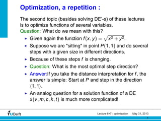
1. Optimization, a repetition :
The second topic (besides solving DE’-s) of these lectures
is to optimize functions of several variables.
Question: What do we mean with this?
◮ Given again the function f(x, y) =
p
x2 + y2.
◮ Suppose we are "sitting" in point P(1, 1) and do several
steps with a given size in different directions.
◮ Because of these steps f is changing.
◮ Question: What is the most optimal step direction?
◮ Answer:If you take the distance interpretation for f, the
answer is simple: Start at P and step in the direction
h1, 1i.
◮ An analog question for a solution function of a DE
x(v, m, c, k, t) is much more complicated!
Lecture 6+7 : optimization May 31, 2013
1
2. Tools for Optimization: partial derivative
To answer the general optimization question, the following
preliminary tools and answers on questions are needed :
Questions:
1. Question1:
Given f(x, y) = sin(x2y3).
Find: ∂ sin(x2y3)
∂x
Find: ∂ sin(x2y3)
∂y
2. Question2:
Given a function g(x, y) and a point P(p0, p1).
What is the meaning of ∂g(P)
∂x > 0
and ∂g(P)
∂y > 0
Lecture 6+7 : optimization May 31, 2013
2
3. Differentiation-rules:
The basic rules for differentiation:
1. Summation rule: (f + g)′ = f′ + g′
2. Product rule: (f · g)′ = f′ · g + f · g′
3. Quotient rule: ( f
g )′ = f′·g−f·g′
g2
4. Chain rule: (f(g(x)))′ = f′(g(x)) · g′(x)
Lecture 6+7 : optimization May 31, 2013
3
5. The meaning of a derivative:
What is meaning of f′(a) > 0?
Some possible answers:
◮ Function f is increasing.
◮ The slope of the tangent-line is positive
The most exact answer is from the definition is:
limh→0
f(a+h)−f(a)
h > 0
Try to understand this value of this answer, why is it better
than former ones?
Lecture 6+7 : optimization May 31, 2013
5
6. The meaning of a partial derivative:
Given a function of 2 variables f(x, y) and a point P(a, b)
The partial derivative of f(P) w.r.p. to x is:
limh→0
f(a+h,b)−f(a,b)
h
notation: ∂f(P)
∂x .
The partial derivative of f(P) w.r.p. to y is:
limh→0
f(a,b+h)−f(a,b)
h
notation: ∂f(P)
∂y .
Lecture 6+7 : optimization May 31, 2013
6
7. The meaning of a partial derivative:
0
(a,€b,€0)
C™
C¡
T¡
P(a,€b,€c)
S T™
z
y
x
Question: In the picture above; determine the sign of ∂f(P)
∂x .
Answer: < 0,
and the sign of ∂f(P)
∂y . Answer: > 0
Remark:
In this picture you see the two tangents belonging to the
partial derivatives. (Both are member of the same tangent
plane)
Lecture 6+7 : optimization May 31, 2013
7
8. Determining a partial derivative:
From these definitions we can deduce that finding the
derivative of a function f(x, y) is nothing more than ordinary
differentiation whereby the other variable is taken constant:
Example 1: ∂
∂x (x2y3) = 2xy3.
Example 2: ∂
∂y (x2y3) = 3x2y2.
Example 3: ∂
∂x
∂
∂y (x2y3)
= 6xy2. A brief notation is
∂2
∂x∂y (x2y3) , a briefer (x2y3)yx .
Lecture 6+7 : optimization May 31, 2013
8
9. The meaning and calculation of a partial
derivative:
(1,€1,€1)
z=4-≈-2¥
(1,€1)
2
y=1
C¡
(1,€1,€1)
z=4-≈-2¥
(1,€1)
2
x=1
C™
z
y
x
z
y
x
Question: In the above
pictures you see the graph of the function f(x, y) = 4 − x2
− 2y2
and the tangents at (1,1,1) belonging to the two partial
derivatives. Find their slopes and are signs of slopes in
accordance with the picture?
answer: fx (x, y) = − 2x, so fx (1, 1) = − 2 so the slope of the first
tangent is -2, so the value of f at (1,1) is decreasing with
increasing x!, which is seen in the picture.
fy (x, y) = − 4y, so fy (1, 1) = − 4 so the slope of the second
tangent is -4, so the value of f at (1,1) is decreasing with
increasing y!, which is also seen in the picture.
Lecture 6+7 : optimization May 31, 2013
9
10. Determining partial derivatives of
f(x1, x2 · · · , xn):
Given f(x1, x2, x3, · · · , xn) = x1
1 x2
2 x3
3 · · · xn
n .
1. Find ∂f
∂x2
2. Given P(1, 1, · · · 1), We take at P a small step in (the
positive) x2-direction and a same small step in (the
positive) x3-direction. In which case is the increase of
f the most? and if we do at P small steps in the
opposite directions?
Further reading and exercises see Stewart 14.3
Lecture 6+7 : optimization May 31, 2013
10
11. Vectors and Lines in R3
, a repetition
Question1:
Given cube C with
A(0, 0, 0), B(1, 0, 0), C(1, 1, 0), D(0, 1, 0), E(0, 0, 1), F(1, 0, 1), G(1, 1, 1), H(0, 1, 1)
1. Find a vector equation for line l1 through A and C.
Answer: l1 = λ1h1, 1, 0i
2. Find a vector equation for line l2 through E and C.
Answer: l2 = h0, 0, 1i + λ2h1, 1, −1i
Lecture 6+7 : optimization May 31, 2013
11
12. Vectors and Lines in R3
, a repetition
Question2:
1. Give the vector equation in R2 of the tangent (line) l of
the graph y = x2 at point P(1, 1).
Answer:l = h1, 1i + λh1, 2i
2. Given the graph of f(x, y) = x2y3 and point P(1, 1, 1)
on it.
Find the vector equations of tangent lines l1 and l2 of
the graph at P in the plane x = 1 and in the plane
y = 1 .
Answer:l1 = h1, 1, 1i + λh0, 1, 3i and l2 = h1, 1, 1i + λh1, 0, 2i
Lecture 6+7 : optimization May 31, 2013
12
13. Directional Derivative
In the last slide we were dealing with tangent lines at a point P in special
directions namely in the x and y direction.
View the next picture:
3
P(x¸, y¸, z¸)
T
y
x
z
In the picture you see a tangent line T in a random direction at P(x0, y0, z0), this
direction is determined by a unit vector u which lies in xy-plane.
Lecture 6+7 : optimization May 31, 2013
13
14. Directional Derivative
We want to calculate the slope, which we note as
Duf(x0, y0), of the tangent line T.
Definition of Duf(x0, y0) :
Duf(x0, y0) = limh→0
f(x0+ah,y0+bh)−f(x0,y0)
h
hereby is u = ha, bi with a2 + b2 = 1, the unit direction.
Question:
Can we calculate Duf(x0, y0) without taking the limit?
Lecture 6+7 : optimization May 31, 2013
14
15. Directional Derivative
Answer:In 4 steps:
1. Question1:
Give the vector equation of the tangent line T
Answer: T = hx0, y0, f(x0, y0)i + λha, b, Duf(x0, y0)i
2. Question2:
Why lie the three space vectors v = ha, b, Duf(x0, y0)i,
v1 = h1, 0, fx (x0, y0)i and v2 = h0, 1, fy (x0, y0)i in one plane?
Answer: They are direction vectors of three tangent lines of the graph of f at point
P(x0, y0, f(x0, y0)). so they lie all in the tangent plane
3. Question3:
Write v as a (linear) combination of v1 and v2.
Answer: v = av1 + bv2
4. Question4:
Express Duf(x0, y0) in fx (x0, y0) and fy (x0, y0)
Answer: From last answer follows Duf(x0, y0) = afx (x0, y0) + bfy (x0, y0)
5. So Duf(x0, y0) = afx (x0, y0) + bfy (x0, y0)
Lecture 6+7 : optimization May 31, 2013
15
16. Directional Derivative: an exercise
Back to our two dimensional distance function:
1. Given f(x, y) =
p
x2 + y2 and P(1, 1). Calculate
Duf(P) for the unit-steps u = h1, 0i, u = h0, 1i and
u = h 1
√
2
, 1
√
2
i
Answer: Dh1,0if(P) = 1
√
2
, Dh0,1if(P) = 1
√
2
, D
h 1
√
2
, 1
√
2
i
f(P) = 1
2. Calculate Duf(P) for the general unit step
u = hcos(θ), sin(θ)i
Answer: Dhcos θ,sin θif(P) = 1
√
2
(cos θ + sin θ)
3. For which θ in the last problem is Duf(P) a maximum?
Answer: θ = π
4
For more exercises and theory see Stewart 14.7
Lecture 6+7 : optimization May 31, 2013
16
17. Dot product:a Repetition
Given two vectors a = ha1, a2i and b = hb1, b2i
Do you remember:
a·b = a1b1 + a2b2
and
a·b = |a||b| cos(θ)
whereby θ is the angle between the given vectors.
What has this to do with:
Duf(x0, y0) = afx(x0, y0) + bfy(x0, y0)
Lecture 6+7 : optimization May 31, 2013
17
18. a convenient formula for Duf(x0, y0)
Duf(x0, y0) = hfx (x0, y0), fy (x0, y0)i·ha, bi.
and
Duf(x0, y0) = |hfx (x0, y0), fy (x0, y0)i||ha, bi| cos(θ).
In the last formula is θ angle between vectors u = ha, bi and hfx (x0, y0), fy (x0, y0)i
Because u = 1 (unit vector) we get
Duf(x0, y0) = |hfx (x0, y0), fy (x0, y0)i| cos(θ)
We note hfx (x0, y0), fy (x0, y0)i as ∇f(x0, y0) and is called the gradient of f at point
(x0, y0).
Lecture 6+7 : optimization May 31, 2013
18
19. An important interpretation of the
gradient.
Look at
Duf(x0, y0) = |∇f(x0, y0)| cos(θ)
Again the question: In which direction u is Duf(x0, y0) a
maximum?
answer: the gradient direction
Some questions:
1. In what direction do you have to take your (unit) step for
minimizing Duf(x0, y0)?
2. and in what direction do you have to take your (unit)
step(s) such that value f(x0, y0) is unaffected?
3. Make a walk in the xy-plane which minimize in every
step the value of
p
x2 + y2!
Lecture 6+7 : optimization May 31, 2013
19
20. A gradient-plot.
In next picture you see a Maple constructed gradient plot for the
function f(x, y) =
p
x2 + y2:
If you follow the opposite gradient vectors starting at a random
point you always end at (0, 0) which belongs to the minimum
value of f.
Lecture 6+7 : optimization May 31, 2013
20
21. Generalizations:
◮ In Rn (n the input variables x1, x2...xn are involved) the
directional derivative is calculated as:
Duf(p) = ∇f(p)·u
◮ with u = hu1, · · · uni a vector in Rn,
◮ with p = hp1, · · · pni a vector in Rn,
◮ with ∇f(p) = hfx1
(p), fx2
(p), · · · fxn (p)i,
◮ with dot product a·b defined as
a1b1 + a2b2 + · · · + anbn,
◮ Interpretation for gradient ∇f(p) is:
If we choose u as ∇f(p)
|∇f(p)| then for given p is Duf(p) a
maximum
◮ Remark: The the gradient vector lives in the input
space (domain).
Lecture 6+7 : optimization May 31, 2013
21
22. An Example.
Question
Given a rectangular box with sizes 8[m] for the length l, 4[m]
for width w and 2[m] for height h.
We change l, w and h such that △l, △w, △h fulfill the
condition:
q
(△l)2 + (△w)2 + (△h)2 = 1.
Estimate which h△l, △w, △hi gives largest volume?
Lecture 6+7 : optimization May 31, 2013
22
23. An Example.
Answer:
◮ We consider the volume V as
function:V(l, w, h) = l · w · h.
◮ We are sitting in P(8, 4, 2).
◮ ∇V = hwh, lh, lwi so in P this equals to h8, 16, 32i
◮ So DuV(8, 4, 2) is a maximal for u = h 1
√
21
, 2
√
21
, 4i
√
21
i
A good estimate is △l = 1
√
21
, △w = 2
√
21
, △l = 4
√
21
.
Lecture 6+7 : optimization May 31, 2013
23
24. Approximating extreme values with the
gradient
Given some function f(x1, · · · xn).
1. Look for a suitable starting point (q1, q2, · · · qn) (in the
domain)
2. Choose a suitable stepsize S (some positive number)
3. Define recursion relation (vector form)
Xn = Xn−1 ± S∇f(Xn−1)
with starting value X0 = hq1, q2, · · · qni. Herein we
choose + if we are looking for a maximum, we choose
− if we are looking for a minimum.
For application see Maple Demo
Lecture 6+7 : optimization May 31, 2013
24