Adaptive combinational filters

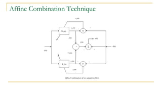
1. Affine Combination Technique
Affine Combination of two adaptive filters
W1(n)
W2(n)
+
∑
∑
∑
x(n)
λ(n)
1-λ(n)
y(n)
y2(n)
e2(n)
y1(n)
e1(n)
d(n)
e(n)
+
+
+
-
-
-

2. Contd…
 The outputs of the two filters are combined using the
mixing parameter, λ(n).
 The overall output of the combined filter is given as
where,
 This combination approach provides robustness against
systems with varying degrees of sparsity and also achieves
better performance than each of the combining filters
separately.

3. Mixing Parameter, λ(n)
 The a priori error signal is defined as
 λ(n) is obtained by minimizing the mean square of the a priori error. The
derivative of with respect to λ(n) is given by
 Setting the derivative to zero results in
 Exponential smoothing:

4.  𝑦 𝑛 = 𝒙𝑇(n)𝐰(𝑛)
 𝑒 𝑛 = 𝑑 𝑛 − 𝑦(𝑛)
 The normalized LMS (NLMS) filter coefficient vector is updated
according to
where, 𝛼 𝑖𝑠 𝑡ℎ𝑒 𝑠𝑡𝑒𝑝 𝑠𝑖𝑧𝑒
 To avoid division with zero, we add a small constant δ
NLMS Adaptive Filter
)
(
)
(
)
(
)
(
)
1
(
2
n
x
n
e
n
x
n
w
n
w




)
(
)
(
)
(
)
(
)
1
(
2
n
x
n
e
n
x
n
w
n
w







5. Improved Proportionate-Normalized
Least Mean Square (IPNLMS)
Improved Proportionate NLMS (IPNLMS) Algorithm
Initialization:
Parameters:
Error:
Update:



 1
L
0
i
i
l
l
(n)
p
L
1
(n)
p
(n)
q
ε
h(n)
2
(n)
h
k)
(1
2L
k
1
(n)
p
1
l
l





1
k
1 


k)/2L
(1
2
x
σ
δIPNLMS 


6. Comparison of NLMS, IPNLMS, CIPNLMS

7. Comparison of APA, IPAPA, CIPAPA
7