mathematics

Instructor: Philip Parzygnat
Introduction
Computer Algebra Systems Modern com-
puters have helped scientists in research and ex-
perimentation since their invention in the mid 20th
century. The computer is a tool that simplifies
many tasks and accomplishes some that we may
find difficult to accomplish using our own insight.
Computer Algebra Systems are a collection of
tools that mathematicians (and other scientists)
use to understand and solve computational prob-
lems. The tools are provided in the form of a
software package and are distributed for general
use. The CAS employed in this course is called
Mathematica. Mathematica was conceptualized by
Stephen Wolfram (a famous mathematician in his
own right). After developing the first version of
Mathematica, Wolfram went on to found a very
successful research and software development com-
pany. A link to his website is available as a link on
the course website (similarly a link to his research
and educational site called MathWorld at Wolfram is also available). Mathematica is a tool you as stu-
dents can use to both solve and visualize math problems. The requirement for solving and visualizing
problems using Mathematica is to understand how the software works and learn the symbolic language
that is required to command the software to execute instructions.
Precalculus and Beyond This course will be structured to help you understand some of your work in
precalculus and introduce you to applications of elementary mathematics. The course may also introduce
you to some new topics that go beyond your precalculus course and start building your intuition of
calculus. We will be focusing on visualizing functions and solving equations (some topics deal with
applications of mathematics to real world problems). Mathematics is a key field to any scientific research
because we are finding (as a people) that more and more phenomena in nature and beyond obey strict
rules that can be described mathematically. With that said I hope the course introduces everyone to the
power of mathematics in general and computers in particular.
1

About Numbers
Defining Mathematics The study of mathematics can be challenging to fully define. One concept
that is unavoidable when studying elementary mathematics is the concept of quantity which is measured
using numbers. A good way to grasp what we study as mathematicians is to understand the underlining
systems that are utilized in the art. Numbers are grouped into classifications in mathematics. The
classifications are based on properties that certain numbers satisfy. Some number classifications describe
numbers that are intuitively harder to grasp. We will discuss one such number (π) in the future.
The Natural Number System Of all numbers (possibly) the easiest to consider is the number 1.
From 1 we can begin to count items (enumerate) using what is called the Natural number system (N).
Counting leads from 1 to 2 and from 2 to 3 etc. therefore the Natural number system can be defined as
follows:
N = {1, 2, 3, ...}
The study of Natural numbers led mathematicians to consider subclasses of the Natural numbers, in
particular (i.) the odd numbers which are not evenly divisible by 2 (ii.) the even numbers which are
all evenly divisible by 2 (iii.) the prime numbers which are only evenly divisible by 1 and themselves
(iv.) perfect squares which can be composed by multiplying a particular natural number by itself (i.e.
2 × 2 = 4). These subclasses are (generally) viewed to have less members than the Natural numbers and
are composed of a subset of the Natural numbers (therefore an even number is also a Natural number
but a Natural number is not necessarily even).
Zero The number 0 was not understood as people began to count, only much later did we decide to
consider the number 0 (which symbolizes the absence of something). The Natural numbers including 0
are called the Whole numbers.
The Integers Once Natural numbers were understood some mathematicians considered the negative
counterparts of particular Natural numbers (i.e. −1 is the negative counterpart to 1). They began using
a system of numbers that included the Natural numbers, zero, and the set of negative counterparts. This
system is called the Integer number system.
1

The Real Numbers To understand the Real number system, we must consider the existence of a
portion of something (i.e. half of an apple). Once we begin to consider portions a new and more
complicated number system must be constructed. The Real number system is used to describe Integer
numbers and fractions of Integer numbers. It is split into two separate categories (i.) Rationals are
numbers that can be represented in fractional form with repeating or terminating decimal expansions
(i.e. 1/3 or 0.3333...) (ii.) Irrationals are numbers that have non-repeating and non-terminating decimal
expansions (i.e. π). The two subclasses of the Real number system have no members in common (they
are disjoint), combined they form the Real number system completely.
The Real Interval Consider a line drawn on a piece of paper.
a bcde
0 1
The line can be subdivided at point a and then subdivided further at b etc. The Real number system
can be used to describe any point i on the line. Mathematicians call the collection of points between 0
and 1 a Real interval and consider the collection to be complete.
2

Arithmetic Operators
Addition and Multiplication Once numbers have been appropriately defined and classified, we can
begin to manipulate numbers using operators. The most basic arithmetic operations are defined as addi-
tion (+) and multiplication (×). Both of these operators have their respective counterparts subtraction
(−) and division (÷). In Mathematica we can perform arithmetic operations without understanding the
symbolic language Mathematica requires to write statements. These basic operations can be executed
more intuitively than most other commands. We can add two numbers by writing the following statement
in Mathematica:
a + b (where a and b are real numbers)
The above statement then needs to be executed or interpreted by Mathematica. In order to execute a
command in Mathematica it is necessary to press the shift key and the enter key at the same time. The
above statement can be written as follows (less intuitive but utilizes Mathematica syntax or the symbolic
language):
Sum[a,b] (where a more general statement could be written Sum[a, b, c, ...])
The remaining arithmetic operations are defined similarly (÷ and × are written / and * respectfully).
Mathematica Statements Mathematica requires an understanding of some basic programming con-
cepts. When we work with computers we must understand that computers are in general very precise
machines and as such are very poor interpreters. Here is an example scenario that explains the point:
In the afternoon, a pedestrian takes a walk into town. He forgets his watch at home and asks another
pedestrian for the time. The pedestrian responds, saying it is 5. Being that it is the afternoon, it is clear
that it is 5pm. If a computer were to ask for the time our response would have to be 5pm (not 5)
because the computer does not have any further intuition.
The idea that we must direct a computer to carry out instructions exactly by writing precise statements
is very important when programming. The rules by which a computer interprets statements is called
syntax.
1

Advanced Examples Below is an example of a complex program written in Mathematica. The ob-
jective of this class will be to reproduce the code for this program with no syntactical errors (i.e. typing
the program into Mathematica exactly as it is on this page).
sieve[n_]:=
Module[{primes=Range[n], s=2}, primes[[1]]=0;
While[s<n+1, Do[primes[[i]]=0, {i, 2s, n, s}]; s=s+1;
While[s<n+1 && primes[[s]]==0, s=s+1]];
DeleteCases[primes, 0]]
2

The Line
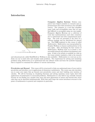
Cartesian Coordinates In geometry the most
basic concept is that of a point. If we draw two
points on a plane (or a piece of paper), these two
points can be interpreted as the two defining points
of a line. In other words, to draw a line we can
connect the two points. The point and line are
the subject matter of the first two definitions in
a well known text in ancient mathematics called
The Elements by Euclid. The text was and is fun-
damental to understanding geometry (in fact the
standard geometric plane is named after Euclid i.e.
the Euclidean plane). Later in history a math-
ematician and philosopher named Rene Descartes
developed Euclid’s ideas into what we now call an-
alytic geometry. In analytic geometry we consider
our geometric objects (i.e. lines or parabolas) to
be imposed in a Cartesian coordinate system (the
x and y axis). Once we impose our geometric ob-
jects in a coordinate system we can begin to algebraically define the objects with respect to the two (or
more) axes. Namely, y = x can be interpreted geometrically and drawn on a Euclidean plane. More
complex figures can also be associated with a particular algebraic form (i.e. the circle x2
+ y2
= 1).
The Conversion Lines are generally written in f(x) form, where (f(x) denotes the y axis). A function
f(x) = mx+b is what we call the general form of a line. A specific line would be described by associating
m and b with real values (i.e. f(x) = 1
2 x + 3). The line f(x) = 1
2 x + 3 is distinct and unique (i.e. any
other line that is reducible to the same form is the same line). For further details on lines consult your
precalculus textbook.
Plotting Lines Mathematica has a method by which we may plot lines (and other geometric objects).
The following is an example of a statement that plots a line in general form:
Plot[mx + b, {x , -10, 10}]
The example above does not work until we substitute m and b with real values.
1

Beyond Analytic Geometry Once we have become familiar with analytic geometry, a more advanced
form of mathematics can be applied to studying geometric objects. Calculus was invented independently
by two men (Newton and Leibniz). Newton wrote about calculus methods in his work Principia and
Leibniz wrote about calculus in a separate work. Calculus helps us understand how geometric objects
are related to their areas and vice versa. When given a line f(x) = 1
2 x + 3, we can integrate (integration
is a process in calculus) f(x) and the result of our integration will be the area under the line. Integration
has a counterpart called differentiation. When we differentiate a line we arrive at the slope (or rate of
change) of the line. These two processes will be briefly described in a future handout and lecture.
2

Geometry
A
B
C
A + B = C2 2 2
The Pythagorean Theorem There exists a re-
lationship between the two sides and hypotenuse
of a right triangle known as the Pythagorean the-
orem. In fact, this is the oldest known theorem
in mathematics. The Pythagorean theorem states
that the hypotenuse c of a right triangle is related
to the two sides of a right triangle by the formula
c2
= a2
+ b2
. A more general rule known as the
law of cosines c2
= a2
+b2
−2abcos(C). The law of
cosines considers a triangle that is not necessarily
right.
Quadratics Quadratic equation are generally
written ax2
+ bx + c. When geometrically trans-
lated these equations are described by parabolas.
In general the functions we study in precalculus
are mostly described when considering the cross
section of a conic. For further details on conics
and conic sections see your precalculus text book.
We can plot quadratic equations using the same
method as we used for plotting lines. We must simply replace the line equation with that of a quadratic.
In order to plot more than one function in a single graph the following statement can be used:
Plot[{f, g, h}, {x , -10, 10}]
In the above statement you must replace f, g, and h with actual functions.
Roots When dealing with quadratic equations there exists a formula for determining the roots of
quadratic equations. This is called the quadratic formula −b±
√
b2−4ac
2a . Geometrically the roots of an
equation describe the x-intercepts of that particular quadratic. In many cases the roots are not real
(they fall into a higher number classiﬁcation called the Complex number system). Below is an example
of a Mathematica statement that solves for the roots of a given quadratic equation.
Solve[ax +bx+c==0, x]2
The above is a general solution. In order to solve for the roots of a quadratic you must replace a, b, and
c with real values.
1

Complex Numbers When solving for the roots of quadratic equations, many solutions have
√
−1 as
a factor.
√
−1 is often written as i or the imaginary number. The standard form for writing complex
numbers is in parts. Complex numbers have both a real and imaginary part (i.e. α + βi). When
multiplying complex numbers we must consider that
√
−1 ×
√
−1 = −1. This caveat has interesting
eﬀects on how these numbers behave. Complex numbers can be geometrically interpreted as points on
a plane. In Cartesian coordinates they are points in two dimensions (i.e. the real dimension and the
imaginary dimension). The plane that we plot complex numbers on is called the Argand plane.
2

Trigonometry
Some Properties Similar to the Pythagorean theorem a2
+b2
= c2
is the Pythagorean (trigonometric)
identity sin2
(x) + cos2
(x) = 12
. sin(x) and cos(x) are trigonometric functions that relate the angles of a
triangle to the perimeter of a triangle. Geometrically, both the sine and cosine curves are periodic over
2π (i.e. repetitive over the interval). Some properties of sine and cosine are known as the amplitude (α),
the frequency (β), the period (γ). The sine function can be defined f(x) = αsin(βx ± γ) (the cosine can
be defined similarly. Now, the amplitude is geometrically interpreted as the height of the curve. The
frequency is geometrically interpreted as the number of periods (repetitions) over the interval. Finally,
the period is geometrically interpreted as the curves offset with respect to its standard period (normally
sine starts at 0 and rises and cosine starts at 1 and falls). In order to understand further the properties
of these trigonometric functions please review the precalculus textbook.
Plotting Trigonometric Functions The sine and cosine functions can be plotted in Mathematica
using the same function we use for plotting all other geometric objects. The following is the code necessary
to plot a sine curve and cosine curve respectfully:
Plot[a Sin(b x + c), {x, 0, 2 Pi}]
Plot[a Cos(b x + c), {x, 0, 2 Pi}]
In the above example α = a, β = b, and γ = c (a, b, and c real valued numbers).
1

θ
Figure 1:
Applications A pendulum is a weight sus-
pended by a pivot so that it may swing freely.
Figure 1 is a diagram of a simple pendulum. Here
the following law holds T ≈ 2π L
g where T is the
period of the pendulum, L is the length of the pen-
dulum, and g is the local acceleration of gravity.
Using a pendulum and this law we can approxi-
mate the local acceleration of gravity by measuring
the period T . The pendulum exhibits approximate
simple harmonic motion which is described by the
following equation θ(t) = θ0cos(2πt
T ). That exem-
pliﬁes how some real world phenomena obey rules
that can be described using mathematics. New-
ton pursued understanding the interworking of the
planets with respect to gravity and described his
ﬁndings in his work (Principia) which came to be
known as Newtonian Mechanics. In recent history
Albert Einstein improved (generalized) Newtonian
mechanics in his theory known as relativity.
2

Calculus
Curves and Areas Calculus is the study of
technique in differentiation and integration. In
this section we will discuss the process of integra-
tion. Let us consider the line f(x) = x. The object
of the analysis is to determine the exact area of a
triangle starting at the origin point and extending
to a point on the x axis (say a). So, being that this
is a line we can intuitively say that the area of a
triangle at a = 1 is 1
2 . Similarly, the area of a tri-
angle at a = 2 is 2 (it may be necessary to sketch a
diagram). The formula that denotes the process of
integrating f(x) is
a
0
xdx. In the formula the in-
tegral is denoted by , the lower bound is denoted
by 0, and the upper bound is denoted by a. In
this particular example we set the lower bound to
0 this is the point of origin from which we want to
determine the area under f(x). The upper bound
is the point of termination past which we are not
concerned with the area under f(x). In this simple
example (of polynomial form) the process of integration is carried out as follows: (i.) xn
→ xn+1
(ii.)
xn+1
→ xn+1
n+1 . So then
a
0 xdx = x2
2
a
0
this result simplified is the general formula for calculating the area
underneath f(x) = x. When simplifying we get a2
2 . For further details on this example there is a calculus
link on the website.
Intuition The process of integration is a limiting process. For any function in order to understand
how integration works we must partition the area underneath the curve into rectangles (as in the image
above). As we partition the area into more rectangles we get a closer and closer approximation of the
area under the curve. When the process approaches a limit (i.e. when there is an infinite partitioning)
the area under the curve is precisely calculated. Integration works in that fashion.
Integrating In Mathematica we can integrate an integrable function using the following command:
Integrate[f(x), {x, a, b}]
In the above example f(x) is the function with variable x, a is the lower bound and b is the upper bound.
1

Summation
1+2+..+n = .5(n x n) + .5 n
1
2
2
A proof without words
Sequences In mathematics sequences are or-
dered sets of objects. Each object in a sequence
is associated with an index. A finite sequence
{a1, a2, a3, ...an} is a sequence that has a definite
beginning and definite end. An infinite sequence
{a1, a2, a3, ...} is a sequence that does not termi-
nate. The natural numbers are an infinite sequence
{1, 2, 3, ...}. The prime numbers are also an infi-
nite sequences {2, 3, 5, 7, 11, ...}.
Series We can study sequences and properties
of sequences independently or we can study se-
ries. A series is the sum of the terms of a se-
quence. The series {1 + 2 + 3 + ... + n} is equiv-
alent to n
2 + n2
2 which is known as the closed
form. A proof of this is depicted in the figure
(to the left). When dealing with understand-
ing series often two terms are used. Namely a
series is either divergent or a series is conver-
gent. When we say a series diverges this implies
that as the series grows, the sum of the series
also grows (without bound). When a series con-
verges as it grows, a series approaches a certain
limit.
Geometric Series Here is an example of a convergent series S = {1 + 1
2 + 1
4 + 1
8 + 1
16 + ...}. As S
grows S approaches 2. This example is a variation of the geometric series. In particular this series can
be written in sigma notation as follows:
∞
i=0
1
2i
Sigma Notation Summation is the process of adding a sequence of terms. Sigma notation is used
to represent the summation process in short hand form. We can write
β
i=α ai to denote the sum
{aα + aα+1 + ... + aβ} We call α the lower bound and β the upper bound. ai is called the term.
1

Mathematica In Mathematica the Sum[.] built in function can be used to sum a finite series. In order
to devise a closed form for an infinite series we still must use our intuition. At present computers are
not powerful enough to derive closed forms of infinite series. In fact many mathematicians study this
problem in research. The following is an example of how Sum[.] works for finite series in Mathematica:
Sum[ai, {i, a, b}]
In the above example ai is the term, a is the lower bound, and b is the upper bound.
2

Computers and Recursion
1 2
3 4 5
Recursion
Computers The modern computer is a prod-
uct of late 19th and early 20th century math-
ematics, physics, and engineering. Thinkers
have tried to produce machines that help in
calculations for centuries (i.e. the abacus).
In the early 20th century two major devel-
opments in science occurred (i.) the quan-
tum physical revolution (the development of a
theory of the atom) (ii.) the advent of the
modern computer. Computers are theoretically
founded using a binary logic to represent infor-
mation and definite algorithms to process infor-
mation.
Binary (Boolean) Logic Consider a light
switch which is either on or off. A binary state
works in the same fashion. A binary state has two
identifying values, namely (i.) 1 (ii.) 0. Informa-
tion that is processed by a computer is stored as a
sequence of binary states. (i.e. 01001010). These
binary sequences are further abstracted to form humanly legible information. For example, 8 binary
states can be used to represent characters in the English alphabet (this is known as ASCII encoding).
The name Boolean is often used for binary logic to honour George Boole who first observed many prop-
erties of binary systems.
Algorithms Computers process binary sequences using definite algorithms. Algorithms are loosley
defined as step by step procedures. Algorithms can be trivial (minimal) or very abstract. Here is an
algorithm for selecting all prime numbers from a list of n Natural numbers (the Mathematica version of
this algorithm was discussed in handout 2).
A) List the first n Natural numbers in their natural order.
B) Identify the first number in the ordered list (if the first number is 1 immediately eliminate the
number).
C) Eliminate every number in the full list that is divisible by the selected number.
D) Repeat B and C until no new number is identifiable (i.e. the ent of our full list).
E) The list of numbers that have not been eliminated are the desired result.
Computers are able to process information in a finite number of steps. This implies that all algorithms
have a definite beginning and termination. Algorithms of this variety are called definite of deterministic
processes.
Recursion Recursion is a mathematical method that applies a function continuously to an (initial)
input until a desired result is reached. In particular consider the trivial recursive concept factorial (i.e.
n!). In computing 7! one must computer 7 × 6 × 5 × 4 × 3 × 2 × 1. Recursively, one can compute 7 × 6!
1

where 6! is computed in the same fashion as 7! this process ends with 2×1! where 1! = 1. In other words,
f(7) = 7 × f(6) and f(6) = 6 × f(5) etc. A recursive function descends until a desired limit (base case)
is reached (in this example 1). Upon terminating at the limit the function then ascends to produce the
desired result.
2

mathematics

Recommended

Recommended

More Related Content

What's hot

What's hot (20)

Viewers also liked

Viewers also liked (13)

Similar to mathematics

Similar to mathematics (20)

mathematics