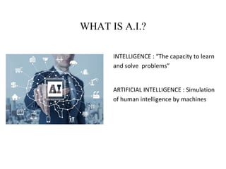
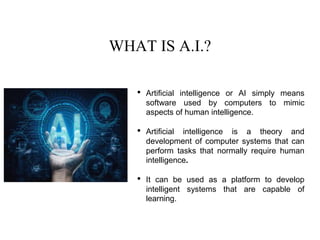
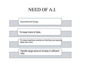
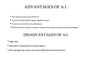
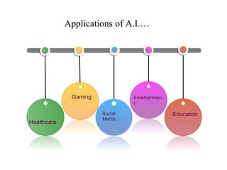
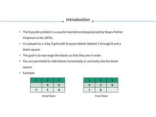
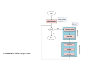
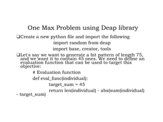
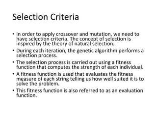
The document provides an introduction to artificial intelligence (AI) and logic programming. It defines AI as simulating human intelligence through machines and discusses what AI is, its advantages and disadvantages, and some applications. It then discusses logic programming, defining it as viewing computation as reasoning over facts and rules. It explains some key concepts in logic programming like facts, rules, predicates, atoms, and unification. It provides examples of using logic programming to match mathematical expressions and validate prime numbers. The document aims to introduce the concepts of AI and logic programming at a high level.


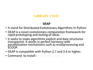
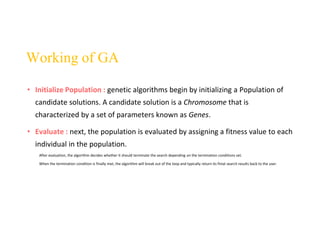
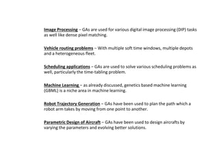
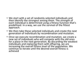
![Matching Mathematical Expressions
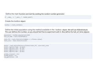
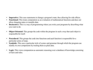
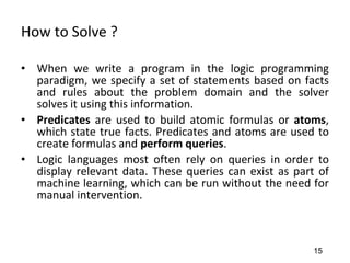
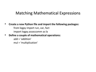
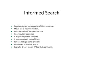
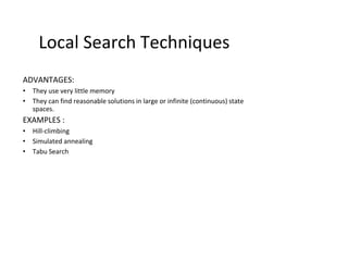
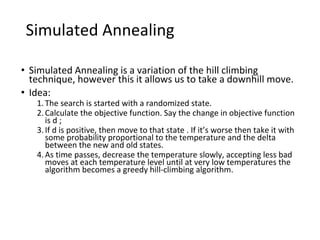
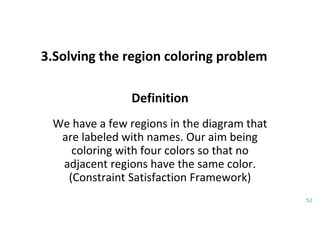
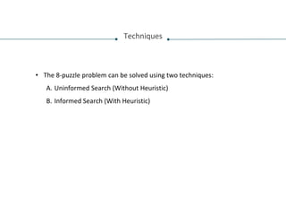
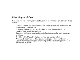
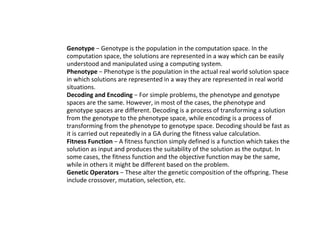
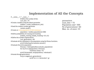
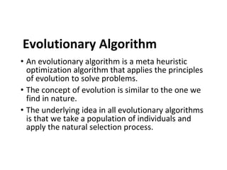
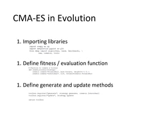
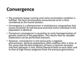
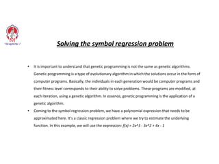
If you observe carefully, all three expressions represent the same
basic expression. Our goal is to match these expressions with the
original expression to extract the unknown values:
expression_og = (add, (mul, 3, -2), (mul, (add, 1, (mul, 2, 3)), -1))
….[ 3 x (-2) + (1 + 2 x 3) x (-1) ]
expression1 = (add, (mul, (add, 1, (mul, 2, a)), b), (mul, 3, c))
….[ (1 + 2 x a) x b + 3 x c ]
expression2 = (add, (mul, c, 3), (mul, b, (add, (mul, 2, a), 1)))
….[ c x 3 + b x (2 x a + 1) ]](https://image.slidesharecdn.com/introductiontoartificialintelligence-240208110313-945a8dec/85/Introduction-to-Artificial-Intelligence-pptx-23-320.jpg)
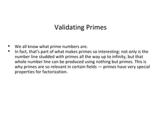
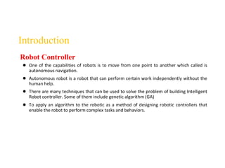
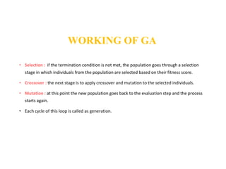
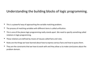
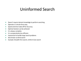
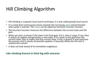
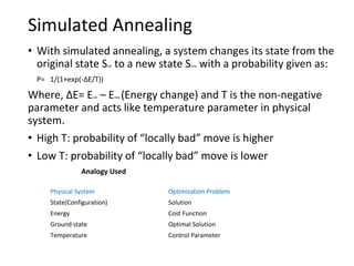
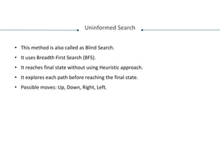
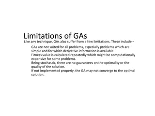
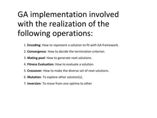
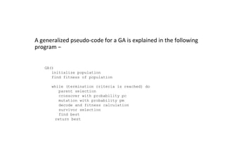
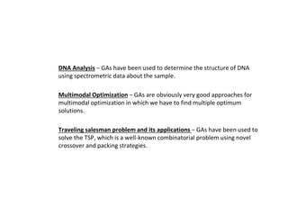
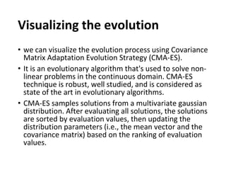
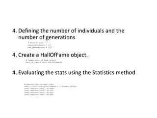
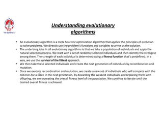
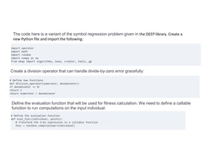
![Validating Primes
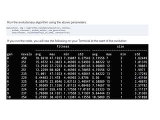
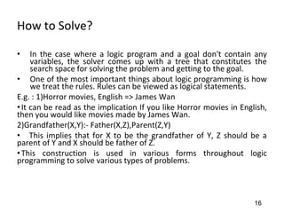
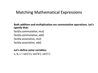
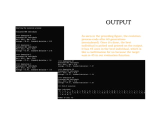
Create a new Python file and import the following packages:
import itertools as it
import logpy.core as lc
from sympy.ntheory.generate import prime, isprime
Method 1 : Check if the elements of x are prime
# def check_prime(x):
if lc.isvar(x):
return lc.condeseq([(lc.eq, x, p)] for p in map(prime, it.count(1)))
else:
return lc.success if isprime(x) else lc.fail
x = lc.var()](https://image.slidesharecdn.com/introductiontoartificialintelligence-240208110313-945a8dec/85/Introduction-to-Artificial-Intelligence-pptx-26-320.jpg)
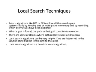
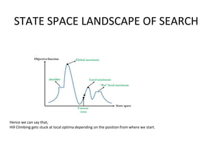

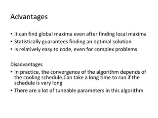

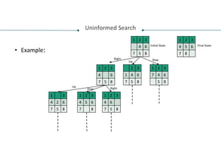

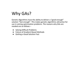
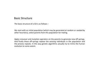
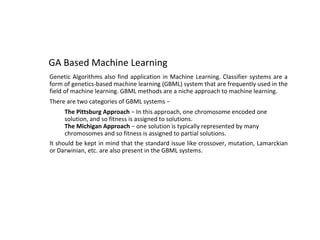
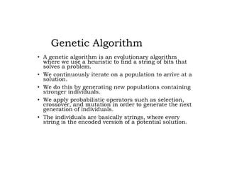
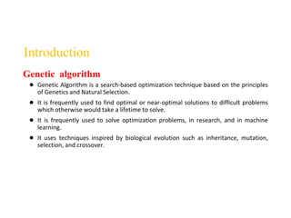
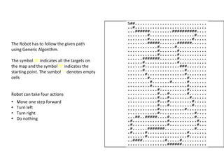
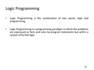
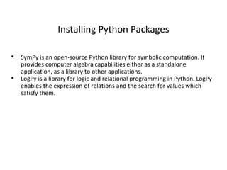
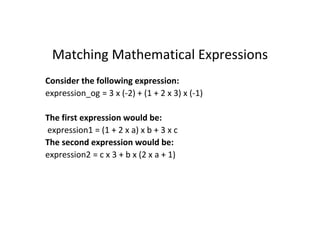
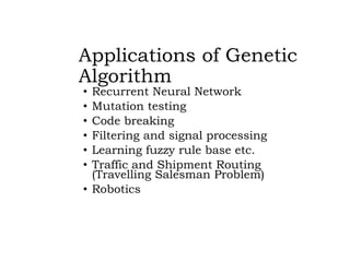
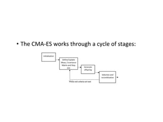
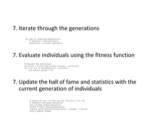
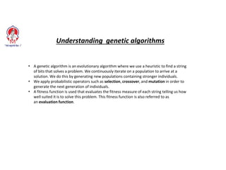
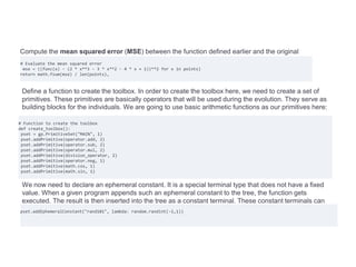
![# Select the next generation individuals
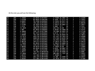
offspring = toolbox.select(population, len(population))
# Clone the selected individuals
offspring = list(map(toolbox.clone, offspring))
# Apply crossover and mutation on the offspring
for child1, child2 in zip(offspring[::2], offspring[1::2]):
# Cross two individuals
if random.random() < probab_crossing:
toolbox.mate(child1, child2)
# "Forget" the fitness values of the children
del child1.fitness.values
del child2.fitness.values
# Apply mutation
for mutant in offspring:
# Mutate an individual
if random.random() < probab_mutating:
toolbox.mutate(mutant)
del mutant.fitness.values](https://image.slidesharecdn.com/introductiontoartificialintelligence-240208110313-945a8dec/85/Introduction-to-Artificial-Intelligence-pptx-90-320.jpg)
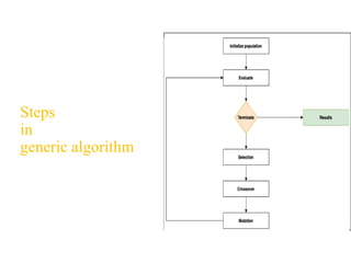
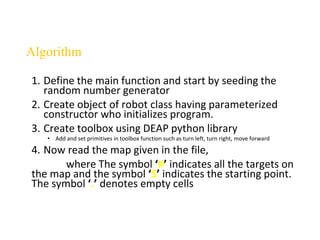
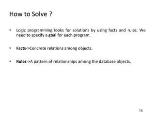
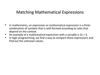
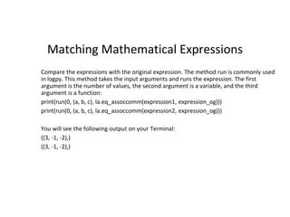
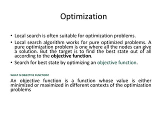
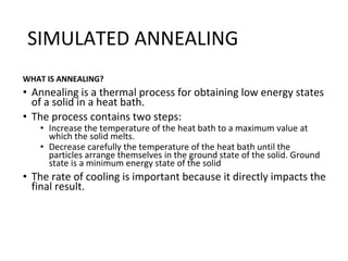
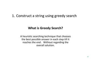
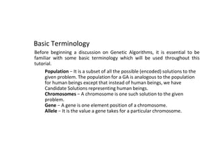
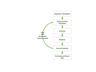
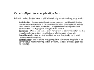
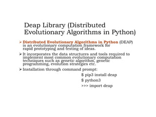
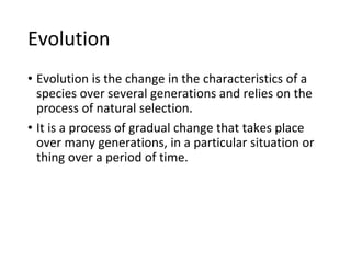
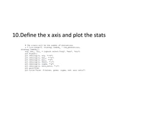
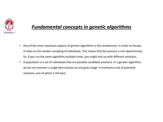
![# Evaluate the individuals with an invalid fitness
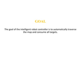
invalid_ind = [ind for ind in offspring if not ind.fitness.valid]
fitnesses = map(toolbox.evaluate, invalid_ind)
for ind, fit in zip(invalid_ind, fitnesses):
ind.fitness.values = fit
print('Evaluated', len(invalid_ind), 'individuals’)
# The population is entirely replaced by the offspring
population[:] = offspring
Print the stats for the current generation to see how it's progressing:
# Gather all the fitnesses in one list and print the stats
fits = [ind.fitness.values[0] for ind in population]
length = len(population)
mean = sum(fits) / length
sum2 = sum(x*x for x in fits)
std = abs(sum2 / length - mean**2)**0.5
print('Min =', min(fits), ', Max =', max(fits))
print('Average =', round(mean, 2), ', Standard deviation =', round(std, 2))
print("n==== End of evolution")
best_ind = tools.selBest(population, 1)[0]
print('nBest individual:n', best_ind)
print('nNumber of ones:', sum(best_ind))](https://image.slidesharecdn.com/introductiontoartificialintelligence-240208110313-945a8dec/85/Introduction-to-Artificial-Intelligence-pptx-91-320.jpg)
![The default name for the arguments is ARGx. Let's rename it x. It's not exactly necessary, but it's a useful feature
that comes in handy:
pset.renameArguments(ARG0='x')
We need to define two object types - fitness and an individual. Let's do it using the creator:
creator.create("FitnessMin", base.Fitness, weights=(-1.0,)) creator.create("Individual", gp.PrimitiveTree,
fitness=creator.FitnessMin)
Create the toolbox and register the functions. The registration process is similar to previous sections:
toolbox = base.Toolbox()
toolbox.register("expr", gp.genHalfAndHalf, pset=pset, min_=1, max_=2)
toolbox.register("individual", tools.initIterate, creator.Individual, toolbox.expr)
toolbox.register("population", tools.initRepeat, list, toolbox.individual)
toolbox.register("compile", gp.compile, pset=pset)
toolbox.register("evaluate", eval_func, points=[x/10. for x in range(-10,10)])
toolbox.register("select", tools.selTournament, tournsize=3)
toolbox.register("mate", gp.cxOnePoint)
toolbox.register("expr_mut", gp.genFull, min_=0, max_=2)
toolbox.register("mutate", gp.mutUniform, expr=toolbox.expr_mut, pset=pset)
toolbox.decorate("mate", gp.staticLimit(key=operator.attrgetter("height"), max_value=17))
toolbox.decorate("mutate", gp.staticLimit(key=operator.attrgetter("height"), max_value=17))
return toolbox](https://image.slidesharecdn.com/introductiontoartificialintelligence-240208110313-945a8dec/85/Introduction-to-Artificial-Intelligence-pptx-114-320.jpg)