Key methods for iron ore price forecasting

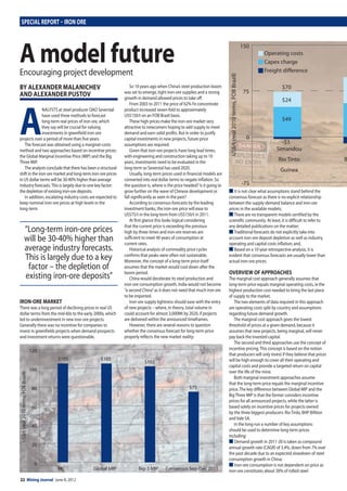
1. 22 Mining Journal June 8, 2012
SPECIAL REPORT – IRON ORE
BY ALEXANDER MALANICHEV
AND ALEXANDER PUSTOV
A
NALYSTS at steel producer OAO Severstal
have used three methods to forecast
long-term real prices of iron ore, which
they say will be crucial for valuing
investments in greenfield iron-ore
projects over a period of more than five years.
The forecast was obtained using a marginal-costs
method and two approaches based on incentive prices:
the Global Marginal Incentive Price (MIP) and the Big
Three MIP.
The analysts conclude that there has been a structural
shift in the iron-ore market and long-term iron-ore prices
in US dollar terms will be 30-40% higher than average
industry forecasts.This is largely due to one key factor:
the depletion of existing iron-ore deposits.
In addition, escalating industry costs are expected to
keep nominal iron-ore prices at high levels in the
long-term.
IRON-ORE MARKET
There was a long period of declining prices in real US
dollar terms from the mid-60s to the early 2000s, which
led to underinvestment in new iron-ore projects.
Generally there was no incentive for companies to
invest in greenfields projects when demand prospects
and investment returns were questionable.
So 10 years ago when China’s steel production boom
was set to emerge, tight iron-ore supplies and a strong
growth in demand allowed prices to take off.
From 2003 to 2011 the price of 62% Fe concentrate
product increased seven-fold to approximately
US$150/t on an FOB Brazil basis.
These high prices make the iron-ore market very
attractive to newcomers hoping to add supply to meet
demand and earn solid profits. But in order to justify
capital investments in new projects, future price
assumptions are required.
Given that iron-ore projects have long lead times,
with engineering and construction taking up to 10
years, investments need to be evaluated in the
long-term so Severstal has used 2020.
Usually, long-term prices used in financial models are
converted into real dollar terms to negate inflation. So
the question is, where is the price headed? Is it going to
grow further on the wave of Chinese development or
fall significantly as seen in the past?
According to consensus forecasts by the leading
investment banks, the iron-ore price will ease to
US$75/t in the long-term from US$150/t in 2011.
At first glance this looks logical considering
that the current price is exceeding the previous
high by three-times and iron-ore reserves are
sufficient to meet 40 years of consumption at
current rates.
Historical analysis of commodity price cycles
confirms that peaks were often not sustainable.
Moreover, the concept of a long-term price itself
assumes that the market would cool down after the
boom period.
China would decelerate its steel production and
iron-ore consumption growth, India would not become
“a second China”as it does not need that much iron ore
to be imported.
Iron-ore supply tightness should ease with the entry
of new projects – where, in theory, total volume in
could account for almost 3,000Mt by 2020, if projects
are delivered within the announced timeframes.
However, there are several reasons to question
whether the consensus forecast for long-term price
properly reflects the new market reality:
■ It is not clear what assumptions stand behind the
consensus forecast as there is no explicit relationship
between the supply-demand balance and iron-ore
prices in the available models;
■ There are no transparent models certified by the
scientific community. At least, it is difficult to refer to
any detailed publications on the matter;
■ Traditional forecasts do not explicitly take into
account iron-ore deposit depletion as well as industry
operating and capital costs inflation; and,
■ Based on a 10-year retrospective analysis, it is
evident that consensus forecasts are usually lower than
actual iron-ore prices.
OVERVIEW OF APPROACHES
The marginal cost approach generally assumes that
long-term price equals marginal operating costs, ie the
highest production cost needed to bring the last piece
of supply to the market.
The two elements of data required in this approach
are operating costs split by country and assumptions
regarding future demand growth.
The marginal cost approach gives the lowest
threshold of prices at a given demand, because it
assumes that new projects, being marginal, will never
pay back the invested capital.
The second and third approaches use the concept of
incentive pricing.This concept is based on the notion
that producers will only invest if they believe that prices
will be high enough to cover all their operating and
capital costs and provide a targeted return on capital
over the life of the mine.
Both marginal investment approaches assume
that the long-term price equals the marginal incentive
price.The key difference between Global MIP and the
BigThree MIP is that the former considers incentive
prices for all announced projects, while the latter is
based solely on incentive prices for projects owned
by the three biggest producers: RioTinto, BHP Billiton
andVale SA.
In the long-run a number of key assumptions
should be used to determine long-term prices
including:
■ Demand growth in 2011-20 is taken as compound
annual growth rate (CAGR) of 3.4%, down from 7% over
the past decade due to an expected slowdown of steel
consumption growth in China;
■ Iron-ore consumption is not dependent on price as
iron-ore constitutes about 30% of rolled-steel
“Long-term iron-ore prices
will be 30-40% higher than
average industry forecasts.
This is largely due to a key
factor – the depletion of
existing iron-ore deposits”
A model futureEncouraging project development
0
20
40
60
80
100
120
Consensus Sep-Dec 2011Big-3 MIPGlobal MIPMC
US$/t(real2010terms,FOBBrazil)
$105 $105
$102
$75
RGP 5Simandou
BHP BilliRio Tinto
AustralGuinea
150
$70
$24
$83
$56
$39
-$12
$49
-$3
Operating costs
Capex charge
Freight difference
75
0
-75
US$/t(real2010terms,FOBBrazil)
22_23MJ120608.indd 22 07/06/2012 09:36

2. June 8, 2012 Mining Journal 23www.mining-journal.comwww.mining-journal.com
production costs and the latter contributes 5-20% of
the final costs of products such as automobiles or
buildings;
■ Excluding China, iron-ore capacity would
have grown at an average level of annual capacity
additions over the last five years: 88Mt.This
equates to 880Mt by 2020, including 90Mt
required to displace China’s inefficient capacity.
However, only 590Mt of this new supply will
come to the international market and participate
in the price setting;
■ China’s government follows rational economic
behaviour and stops domestic iron-ore production if it
is less cost-efficient than imported ore. In our base
scenario, one-third, or 90Mt, of production would be
stopped;
■ Iron-ore prices are determined by a marginal
producer based on a supply curve of international trade
and China’s domestic supply; and,
■ Depletion of existing deposits is assumed at circa
30Mt globally each year, according to McKinsey
estimates, this means that new projects need to deliver
310Mt to the market in the next 10 years simply to
sustain production at current levels.
MARGINAL-COST-BASED FORECASTS
Gauging the 1,760Mt on the supply curve, which
is based on operating costs, the long-term price
comes out at US$105/t, or two-thirds of the price
in 2011.
This marginal cost is due to some high production
costs in China, and at that price the country will
produce 200Mt/y versus around 290Mt/y currently.
Operating costs for new projects are assumed to
equal ex-China weighted average operating costs
as of 2010 due to absence of more precise data.
However, this number could be an underestimate
given that new mines are less cost efficient than old
ones, with operating costs for some new projects in
Australia reaching US$70/t.
If we were to assume that supply and demand grows
at consensus expectations of 5% and 3%, respectively,
long-term prices will fall to US$51/t, but demand could
easily accelerate to 5%, and the iron-ore price would
jump to US$105/t.
Putting these scenarios on a probability matrix and
excluding the unlikely cases of slow demand
and rapid supply growth, the long-term price
would range from US$91/t to US$158/t with a
94% probability considering the correlation of different
scenarios.
The marginal cost approach does not take into
account the capital cost element, which is quite
important for development of new projects.
INCENTIVE PRICE CONCEPT
The incentive price is the level that encourages the
entry of a new project by covering not only operating
costs but also discounted capital investments and a
return on capital.
It should be mentioned that a calculation of
incentive prices for different iron-ore projects also
includes the normalisation to a single base of iron
content, 62% Fe in our case.
The future incentive supply curve was built
using incentive prices for new projects and operating
costs for existing ones.This approach is based on the
assumption that new projects’delivery requires the
forecasted long-term price to be equal or higher than
the incentive price.
Moving on to the specifics, in 2020 iron-ore
demand is projected to account for 1,760Mt,
therefore, the long-term iron-ore price would
equal US$105/t.
This is the same price as derived using the marginal
cost approach, and in fact the marginal producer is one
and the same – China’s high cost iron-ore producer.The
highest incentive price for a new project here is
US$72/t.Therefore, operating costs as well as invested
capital are fully covered for all new capacity.
Again excluding the unlikely cases of slow
demand and rapid supply growth, the long-term price
would range from US$91/t to US$158/t with a 71%
probability (or 94% considering correlation between
scenarios) which is the same as the marginal cost
approach.
So, while the global marginal incentive price
approach is easily explainable and takes capital
investments into accounts, it still has most of the
shortcomings of the marginal cost method:
■ It requires a long-term demand growth assumption,
which is hard to predict correctly;
■ It requires future“incentive”supply curve, which is
built on fragmented data regarding project operational
costs and capital investments;
■ It is highly sensitive to small changes in demand as
the 4th quartile of the supply curve is very steep; and,
■ It assumes the iron-ore market to be in perfect
competition, while it really is an oligopoly.
The next approach, based on the BigThree MIP does
consider the oligopolistic character of the iron-ore
market and does not require demand and supply
projections, as the BigThree are assumed implicitly to
provide this information in making their investment
decisions.
THE BIGTHREE APPROACH
This method assumes that the iron-ore market is an
oligopoly, where RioTinto, BHPB andVale are the most
informed and influential market players controlling 70%
of international trade and are expected to hold this
influence in the long term.Therefore, the incentive price
ofThe BigThree marginal project could be used as a
benchmark for the long-term price.
It also assumes that it is in the interest of the Big
Three to underestimate capital expenditure of new
projects to increase entry barriers for other companies
and get favourable funding.This means that the
approach estimates the lower boundary of the
long-term price.
The long-term price is US$102/t, which is the
incentive price forVale’s Carajas Serra Sul project.
One can see that the marginal incentive price
forecast is almost equal to the long-term price in the
other methods. But it is clear thatVale’s Serra Sul is not
on the future“incentive”supply curve.There are two
possible reasons for this:
Firstly,Vale could have more optimistic views on
either demand growth or different views on the set of
new projects coming on stream. For example, they
could assume that the projects being developed by
larger and experienced miners would be realized first,
even if those projects are not the most efficient ones in
terms of incentive price.
Secondly,Vale’s marginal project could be an option
that would be developed only if the market is
favourable. If this is the case, the long-term price would
be downgraded to the incentive price of BHPB’s RGP-5
expansion.
COMPARING LONG-TERM PRICE FORECASTS
In conclusion, the long-term iron-ore price in real 2010
dollar terms would decline from the current level of circa
US$150/t in any of the presented scenarios down to
US$100/t.
The consensus is more than 40% lower than our
estimates, suggesting that forecasts included in the
consensus do not include deposit depletion.This is very
likely to be true because analysts typically do not
explicitly mention this.
While forecasts obtained by all of the approaches are
almost identical, ranging from US$102/t to US$105/t,
butThe BigThree approach seems to be the most
straightforward method.
However, the long-term price forecasts would not
hold true if demand collapses, for example, if China
experiences a hard landing.
To make it more concise, if in the next 10 years
China experiences a 10% reduction of steel
production compared with 2010, the long-
term price would sit on the low marginal cost level
(roughly US$50/t).
Considering different scenarios of supply and
demand and their correlation, the long-term price
would range from $US91/t to US$158/t with a 94%
probability.
Presented forecasts are in real 2010 dollar terms
and so exclude dollar inflation and industry operating
costs escalation (wage growth, local currencies
appreciation, etc).
Using a halved historical industry deflator of 6%,
long-term prices escalate to $US185/t by 2020.This is a
15% growth rate compared with nominal 2011’s
US$160/t. So, the actual probable peak is in nominal
iron-ore prices is yet to come.
Alexander Malanichev is head of strategic marketing at Severstal; Alexander Pustov is senior analyst, strategic marketing, at Severstal
“From 2003 to 2011 the
price of 62% Fe concentrate
product has increased
seven-fold to approximately
US$150/t on an FOB Brazil
basis”
Carajas Serra SulRGP 5
ValeBHP Billiton
BrazilAustralia
$83
$105
$56
$70
$35
$39
-$12
22_23MJ120608.indd 23 07/06/2012 09:36