The t-test compares the means of two groups to determine if they are statistically significantly different from each other. It calculates a t-value based on the difference between the group means (the signal) relative to the variation within each group (the noise). A larger t-value indicates a greater difference between the means relative to the within-group variation, and thus a lower probability the difference is due to chance. The t-test has various applications, including comparing the effectiveness of different medical treatments.

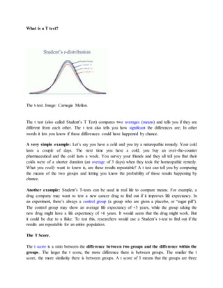
1. What is a T test?
The t-test. Image: Carnegie Mellon.
The t test (also called Student’s T Test) compares two averages (means) and tells you if they are
different from each other. The t test also tells you how significant the differences are; In other
words it lets you know if those differences could have happened by chance.
A very simple example: Let’s say you have a cold and you try a naturopathic remedy. Your cold
lasts a couple of days. The next time you have a cold, you buy an over-the-counter
pharmaceutical and the cold lasts a week. You survey your friends and they all tell you that their
colds were of a shorter duration (an average of 3 days) when they took the homeopathic remedy.
What you really want to know is, are these results repeatable? A t test can tell you by comparing
the means of the two groups and letting you know the probability of those results happening by
chance.
Another example: Student’s T-tests can be used in real life to compare means. For example, a
drug company may want to test a new cancer drug to find out if it improves life expectancy. In
an experiment, there’s always a control group (a group who are given a placebo, or “sugar pill”).
The control group may show an average life expectancy of +5 years, while the group taking the
new drug might have a life expectancy of +6 years. It would seem that the drug might work. But
it could be due to a fluke. To test this, researchers would use a Student’s t-test to find out if the
results are repeatable for an entire population.
The T Score.
The t score is a ratio between the difference between two groups and the difference within the
groups. The larger the t score, the more difference there is between groups. The smaller the t
score, the more similarity there is between groups. A t score of 3 means that the groups are three

2. times as different from each other as they are within each other. When you run a t test, the bigger
the t-value, the more likely it is that the results are repeatable.
 A large t-score tells you that the groups are different.
 A small t-score tells you that the groups are similar.
T-Values and P-values
How big is “big enough”? Every t-value has a p-value to go with it. A p-value is the probability
that the results from your sample data occurred by chance. P-values are from 0% to 100%. They
are usually written as a decimal. For example, a p value of 5% is 0.05. Low p-values are good;
They indicate your data did not occur by chance. For example, a p-value of .01 means there is
only a 1% probability that the results from an experiment happened by chance. In most cases, a
p-value of 0.05 (5%) is accepted to mean the data is valid.
Calculating the Statistic
There are three main types of t-test:
 An Independent Samples t-test compares the means for two groups.
 A Paired sample t-test compares means from the same group at different times (say, one
year apart).
 A One sample t-test tests the mean of a single group against a known mean.
You probably don’t want to calculate the test by hand (the math can get very messy, but if you
insist you can find the steps for an independent samples t test here.
Use the following tools to calculate the t test:
How to do a T test in Excel.
T test in SPSS.
T distribution on the TI 89.
T distribution on the TI 83.
What is a Paired T Test (Paired Samples T Test / Dependent Samples T Test)?
A paired t test (also called a correlated pairs t-test, a paired samples t test or dependent
samples t test) is where you run a t test on dependent samples. Dependent samples are
essentially connected — they are tests on the same person or thing. For example:
 Knee MRI costs at two different hospitals,
 Two tests on the same person before and after training,

3.  Two blood pressure measurements on the same person using different equipment.
When to Choose a Paired T Test / Paired Samples T Test / Dependent Samples T Test
Choose the paired t-test if you have two measurements on the same item, person or thing. You
should also choose this test if you have two items that are being measured with a unique
condition. For example, you might be measuring car safety performance in Vehicle Research and
Testing and subject the cars to a series of crash tests. Although the manufacturers are different,
you might be subjecting them to the same conditions.
With a “regular” two sample t test, you’re comparing the means for two different samples. For
example, you might test two different groups of customer service associates on a business-related
test or testing students from two universities on their English skills. If you take a random sample
each group separately and they have different conditions, your samples are independent and you
should run an independent samples t test (also called between-samples and unpaired-samples).
The null hypothesis for the for the independent samples t-test is μ1 = μ2. In other words, it
assumes the means are equal. With the paired t test, the null hypothesis is that the pairwise
difference between the two tests is equal (H0: µd = 0). The difference between the two tests is
very subtle; which one you choose is based on your data collection method.
Paired Samples T Test By hand
Sample question: Calculate a paired t test by hand for the following data:
Step 1: Subtract each Y score from each X score.
Anatomy of a t-test
A t-test is commonly used to determine whether the mean of a population significantly differs
from a specific value (called the hypothesized mean) or from the mean of another population.
For example, a 1-sample t-test could test whether the mean waiting time for all patients in a
medical clinic is greater than a target wait time of, say, 15 minutes, based on a random sample of
patients.

4. To determine whether the difference is statistically significant, the t-
test calculates a t-value. (The p-value is obtained directly from this t-value.) To find the formula
for the t-value, choose Help > Methods and Formulas in Minitab, then click Basic statistics >
1-sample t > Test statistic. Here's what you'll see:
That jumble of letters and symbols may look like an incantation from a sorcerer’s book.
But the formula is much less mystical if you remember there are two driving forces behind it: the
numerator (top of the fraction) and the denominator (bottom of the fraction).
The Numerator Is the Signal
The numerator in the 1-sample t-test formula measures the strength of the signal: the difference
between the mean of your sample (xbar) and the hypothesized mean of the population (µ0).
Consider the patient waiting time example, with the hypothesized mean wait time of 15 minutes.
If the patients in your random sample had a mean wait time of 15.1 minutes, the signal is 15.1-15
= 0.1 minutes. The difference is relatively small, so the signal in the numerator is weak.

5. However, if patients in your random sample had a mean wait time of 68 minutes, the difference
is much larger: 68 - 15 = 53 minutes. So the signal is stronger.
The Denominator is the Noise
The denominator in the 1-sample t-test formula measures the variation or “noise” in your sample
data.
S is the standard deviation—which tells you how much your data bounce around. If one patient
waits 50 minutes, another 12 minutes, another 0.5 minutes, another 175 minutes, and so on,
that’s a lot of variation. Which means a higher s value—and more noise. If, on the other hand,
one patient waits 14 minutes, another 16 minutes, another 12 minutes, that’s less variation,
which means a lower value of s, and less noise.
What about the √n (below the s)? That’s the square root of your sample size. What that does,
very loosely speaking, is “average” out the variation based on the number of data values in the
sample. So, all things being equal, a given amount of variation is “noisier” for a smaller sample
than for a larger one.
The t-Value: The Ratio of Signal to Noise
As the above formula shows, the t-value simply compares the strength of the signal (the
difference) to the amount of noise (the variation) in the data.
If the signal is weak relative to the noise, the (absolute) size of the t-value will be smaller. So the
difference is not likely to be statistically significant:

6. On the graph at right, the difference between the sample mean (xbar) and the hypothesized mean
(µ0) is about 16 minutes. But because the data is so spread out, this difference is not statistically
significant. Why? The t-value—the ratio of signal to noise—is relatively small due to the large
denominator.
However, if the signal is strong relative to the noise, the (absolute) size of the t-value will be
larger. So the difference between xbar and the µ0 is more likely to be statistically significant:

7. On this graph, the difference between the sample mean (xbar) and the hypothesized mean (µ0) is
the same as on the previous graph—about 16 minutes. The sample size is also the same. But this
time, the data is much more tightly clustered. Due to less variation, the same difference of 16
minutes is now statistically significant!
Statistically Significant Messages
So how is the t-test like telling a teenager to clean up the mess in the kitchen?
If the teenager is listening to music, playing a video game, texting friends, or distracted by any of
the other umpteen sources of "noise" that pervade our lives, the louder and stronger you need to
make your verbal signal to achieve "significance." Alternatively, you could insist on removing
those sources of extraneous noise before you communicate—in which case you wouldn't need to
raise your voice at all.
Similarly, if your t-test results don't achieve statistical significance, it could be for any of the
following reasons:
 The difference (signal) isn't large enough. Nothing you can do about that, assuming
that your study is properly designed and you've collected a representative sample.
 The variation (noise) is too great. This is why it's important to remove or account
for extraneous sources of variation when you plan your analysis. For example, you

8. could use a control chart to identify and eliminate sources of special-cause variation
from your process before you collect data for a t-test on the process mean.
 The sample is too small. Remember the effect of variation is lessened by sample
size. That means for a given difference and a given amount of variation, a larger sample
is more likely to achieve statistical significance, as shown in this graph:
(This effect also explains why an extremely large sample can produce statistically significant
results even when a difference is very small and has no practical consequence.)
By the way, in case you're wondering, these basic relationships are similar for a 2-sample t-test
and a paired t- test. Although their formulas are a bit more complex (see Help > Methods and
Formulas> Statistics> Basic Statistics), the basic driving forces behind them are essentially the
same.
These formulas also explain why statisticians often cringe in response to the language sometimes
used to convey t-test results. For example, a statistically insignificant t-test result is often
reported by stating, “There is no significant difference...”