
Recommended
Recommended
More Related Content
What's hot
What's hot (18)
Similar to Central Bank Intervention and Exchange Rate Volatility
Similar to Central Bank Intervention and Exchange Rate Volatility (20)
More from Nicha Tatsaneeyapan
More from Nicha Tatsaneeyapan (20)
Recently uploaded
Recently uploaded (20)
Central Bank Intervention and Exchange Rate Volatility
- 1. Research Division Federal Reserve Bank of St. Louis Working Paper Series Central Bank Intervention and Exchange Rate Volatility, Its Continuous and Jump Components Michel Beine Jérôme Lahaye Sébastien Laurent Christopher J. Neely and Franz C. Palm Working Paper 2006-031C http://research.stlouisfed.org/wp/2006/2006-031.pdf May 2006 Revised February 2007 FEDERAL RESERVE BANK OF ST. LOUIS Research Division P.O. Box 442 St. Louis, MO 63166 ______________________________________________________________________________________ The views expressed are those of the individual authors and do not necessarily reflect official positions of the Federal Reserve Bank of St. Louis, the Federal Reserve System, or the Board of Governors. Federal Reserve Bank of St. Louis Working Papers are preliminary materials circulated to stimulate discussion and critical comment. References in publications to Federal Reserve Bank of St. Louis Working Papers (other than an acknowledgment that the writer has had access to unpublished material) should be cleared with the author or authors.
- 2. Central Bank Intervention and Exchange Rate Volatility, Its Continuous and Jump Components∗ Michel BEINE† Jérôme LAHAYE‡ Sébastien LAURENT§ Christopher J. NEELY¶ Franz C. PALMk First version: May 2006 Revised: August 2006 This version: February 2007 Abstract We analyze the relationship between interventions and volatility at daily and intra-daily frequencies for the two major exchange rate markets. Using recent econometric methods to estimate realized volatility, we employ bipower variation to decompose this volatility into a continuously varying and jump component. Analysis of the timing and direction of jumps and interventions imply that coordinated interventions tend to cause few, but large jumps. Most coordinated operations explain, statistically, an increase in the persistent (continuous) part of exchange rate volatility. This correlation is even stronger on days with jumps. Keywords: Intervention, jumps, bi-power variation, exchange rate, volatility JEL Codes: F31, F33, C34 ∗The authors thank Mardi Dungey, Mark Taylor and participants at the International Journal of Finance and Economics Conference on central bank intervention for very helpful comments and Justin Hauke for excellent research assistance. This text presents research results of the Belgian Program on Interuniversity Poles of Attraction initiated by the Belgian State, Prime Minister’s Office, Science Policy Programming. The scientific responsibility is assumed by the authors. The views expressed are those of the individual authors and do not necessarily reflect official positions of the Federal Reserve Bank of St. Louis, the Federal Reserve System, or the Board of Governors. †University of Luxembourg and Free University of Brussels; mbeine@ulb.ac.be ‡CeReFiM, University of Namur and CORE; Jerome.Lahaye@fundp.ac.be §CeReFiM, University of Namur and CORE; Sebastien.Laurent@fundp.ac.be ¶Assistant Vice President, Research Department, Federal Reserve Bank of St. Louis; neely@stls.frb.org kMaastricht University, Faculty of Economics and Business Administration and CESifo; F.Palm@ke.unimaas.nl 1
- 3. 1 Introduction During a period of twenty years (1985-2004), the central banks of the U.S., Japan and Germany (Europe) intervened more than 600 times in either the DEM-dollar (DEM/USD or EUR/USD after the introduction of the euro) or the yen-dollar (JPY/USD) market. On average, they intervened almost three times per month. It is not surprising that central banks should frequently intervene in markets that are of crucial importance for international competitiveness. Given the importance of understanding foreign exchange markets, for scientific and policy reasons, one would like to assess the impact of central bank interventions (CBIs hereafter) on exchange rates. The large empirical literature on the impact of CBIs provides mixed evidence on the impact of CBI on exchange rate returns. In general, authors fail to identify effects on the conditional mean of exchange rate returns at a daily frequency (Baillie and Osterberg 1997). When effects on the spot exchange rate returns are detected, they are often found to be perverse, i.e. purchases of U.S. dollar leading to a depreciation of the dollar (Baillie and Osterberg 1997, Beine, Bénassy- Quéré, and Lecourt 2002). This perverse result tends to hold for both unilateral and coordinated interventions. This result has usually been interpreted as indicating a lack of credibility, or ascribed to inappropriate identification schemes in the presence of leaning-against-the-wind policies (Neely 2005b). Recent studies conducted at intra-daily frequencies nevertheless find that CBIs can move the exchange rate, at least in the very short run (Fischer and Zurlinden 1999, Dominguez 2003). The empirical literature is much more conclusive with respect to the impact of CBIs in terms of exchange rate volatility. Most studies conclude that intervention tends to increase exchange rate volatility (Humpage 2003) and this result is robust to the use of any of the three main mea- sures of asset price volatility: univariate GARCH models (Baillie and Osterberg 1997, Dominguez 1998, Beine, Bénassy-Quéré, and Lecourt 2002); implied volatilities extracted from option prices (Bonser-Neal and Tanner 1996, Dominguez 1998, Galati and Melick 1999); and realized volatility (Beine, Laurent, and Palm 2005, Dominguez 2004). This paper looks at the relation between intervention and the components of volatility. We in- vestigate how CBIs affect the continuous, persistent part of exchange rate volatility and the discon- tinuous component. Our approach relies on bi-power variation (Barndorff-Nielsen and Shephard (2004, 2006)) to decompose exchange rate changes into a continuous part and a jump compo- nent. Bi-power variation consistently estimates the continuous volatility even in the presence of jumps (i.e. for a continuous-time jump diffusion process). And the realized volatility (sum of 2
- 4. squared intradaily returns) consistently estimates the sum of both the continuous volatility and the discontinuities (jumps) in the underlying price process. Therefore the difference between real- ized volatility and the bi-power variation consistently estimates the contribution to the quadratic variation process due to the discontinuities (jumps). Barndorff-Nielsen and Shephard (2006) suggest that jumps in foreign exchange markets are linked to the arrival of macroeconomic news, in line with the results of Andersen, Bollerslev, Diebold, and Vega (2003). In this respect, our findings illuminate the importance of interventions for explaining the dynamics of exchange rates and the extent to which interventions impact rates similarly to macroeconomic news. Our investigation covers central bank activity on the two largest exchange rate markets. We focus on Fed, Bundesbank (ECB after 1998) and Bank of Japan interventions over the last twenty years. Using the method of bi-power variation with 5-minute exchange rate data, we identify the days in which exchange rates jumps occur. This allows us to investigate whether intervention days are associated with the occurrence of these jumps. To achieve this goal, we proceed in five steps. First, we decompose realized volatility into a continuous component and a jump component. We investigate the relationship between CBIs and discontinuities in the JPY/USD and USD/EUR markets and find that while jumps are not more likely to occur on days of intervention, the jumps that do occur are larger than average. In particular, only a few coordinated interventions could reasonably generate jumps. Coordinated CBIs do predict the smooth, persistently varying component of realized volatility, however. Second, to check for the direction of causality between jumps and coordinated CBIs, we care- fully study the number of jumps and the timing of their occurrence during the CBI days. Most of the jumps on CBI days occurred during or after the overlap of European and U.S. markets, when most coordinated interventions take place. We then examine the direction of the jumps and coordinated CBIs for days on which they both occur. This analysis strongly suggests that inter- vention normally generates the jumps, rather than reacting to them. The only period in which intervention appears to respond to jumps is that of the ”Louvre Accords,” when central banks were very keen to dampen volatility by leaning against the wind. Third, to control for the impact of macroeconomic announcements on exchange rate volatility, we check for the joint occurrence of jumps, coordinated interventions on the corresponding for- eign exchange markets and of macroeconomic announcements. For the JPY/USD, macroeconomic 3
- 5. announcements were made on half of the 14 days where jumps occurred and a coordinated in- tervention took place in this market. For the USD/EUR market, macroeconomic announcements occurred only on three out of 10 days with jumps in the exchange rate and a coordinated inter- vention. The timing evidence suggests that a subset of jumps on these days were not the result of macroeconomic announcements. Instead, some coordinated interventions might be the primary cause of the observed discontinuities. Fourth, a formal regression analysis confirms these findings. Fifth, we discuss the economic interpretation of the findings, the implications for foreign ex- change market policy of central banks and some extensions of the methodology. The paper is organized as follows. Section 2 details the procedure used to identify the jump components of the realized volatilities. Section 3 provides some details on the data. Section 4 reports our empirical analysis relating the occurrence of jumps with CBIs while Section 5 proposes an interpretation of the main findings. Finally, Section 6 concludes. 2 Extracting the jump component Let p(t) be a logarithmic asset price at time t. Consider the continuous-time jump diffusion process dp(t) = µ(t)dt + σ(t)dW(t) + κ(t)dq(t), 0 ≤ t ≤ T, (1) where µ(t) is a continuous and locally bounded variation process, σ(t) is a strictly positive stochastic volatility process with a sample path that is right continuous and has well defined limits, W(t) is a standard Brownian motion, and q(t) is a counting process with intensity λ(t) (P[dq(t) = 1] = λ(t)dt and κ(t) = p(t) − p(t−) is the size of the jump in question). The quadratic variation for the cumulative process r(t) ≡ p(t)−p(0) is the integrated volatility of the continuous sample path component plus the sum of the q(t) squared jumps that occurred between time 0 and time t: [r, r]t = Z t 0 σ2 (s)ds + X 0<s≤t κ2 (s). (2) Now, let us define the daily realized volatility as the sum of the corresponding intradaily squared returns: RVt+1(∆) ≡ 1/∆ X j=1 r2 t+j∆,∆, (3) 4
- 6. where rt,∆ ≡ p(t) − p(t − ∆) is the discretely sampled ∆-period return.1 So 1/∆ is the number of intradaily periods (288 in our application). In order to disentangle the continuous and the jump components of realized volatility, we need to consistently estimate integrated volatility, even in the presence of jumps in the process. This is done using the asymptotic results of Barndorff-Nielsen and Shephard (2004, 2006). Barndorff-Nielsen and Shephard (2004) show that the realized volatility converges uniformly in probability to the increment of the quadratic variation process as the sampling frequency of the returns increases (∆ → 0):2 RVt+1(∆) → Z t+1 t σ2 (s)ds + X t<s≤t+1 κ2 (s). (4) That means that realized volatility consistently estimates integrated volatility as long as there are no jumps. The realized bi-power variation is defined as the sum of the product of adjacent absolute intradaily returns standardized by a constant: BVt+1(∆) ≡ µ−2 1 1/∆ X j=2 |rt+j∆,∆||rt+(j−1)∆,∆|, (5) where µ1 ≡ p 2/π ' 0.79788 is the mean of the absolute value of a standard normally distributed random variable. It can indeed be shown that even in the presence of jumps, BVt+1(∆) → Z t+1 t σ2 (s)ds. (6) Thus, the difference between the realized volatility and the bi-power variation consistently estimates the jump contribution to the quadratic variation process. When ∆ → 0: RVt+1(∆) − BVt+1(∆) → X t<s≤t+1 κ2 (s). (7) Moreover, because a finite sample estimate of the squared jump process might be negative (in Equation (7)), we truncate the measurement at zero, i.e. Jt+1(∆) ≡ max[RVt+1(∆) − BVt+1(∆), 0]. (8) One might wish to select only statistically significant jumps, to consider very small jumps to be part of the continuous sample path rather than genuine discontinuities. The Barndorff-Nielsen 1We use the same notation as in Andersen, Bollerslev, and Diebold (2005) and normalize the daily time interval to unity. We drop the ∆ subscript for daily returns: rt+1,1 ≡ rt+1. 2See also, for example, Andersen and Bollerslev (1998a), Andersen, Bollerslev, Diebold, and Labys (2001), Barndorff-Nielsen and Shephard (2002a), Barndorff-Nielsen and Shephard (2002b), Comte and Renault (1998). 5
- 7. and Shephard (2004, 2006) results, extended in Barndorff-Nielsen, Graversen, Jacod, Podolskij, and Shephard (2005), imply:3 RVt+1(∆) − BVt+1(∆) q (µ−4 1 + 2µ−2 1 − 5)∆ R t+1 t σ4(s)ds → N(0, 1), (9) when there is no jump and for ∆ → 0, under sufficient regularity conditions. We need to estimate the integrated quarticity R t+1 t σ4 (s)ds to compute this statistic. The realized tri-power quarticity measure permits us to estimate it consistently, even in the presence of jumps: TQt+1(∆) ≡ ∆−1 µ−3 4/3 1/∆ X j=3 |rt+j∆,∆|4/3 |rt+(j−1)∆,∆|4/3 |rt+(j−2)∆,∆|4/3 , (10) with µ4/3 ≡ 22/3 Γ(7/6)Γ(1/2)−1 . Thus, we have that, for ∆ → 0: TQt+1(∆) → Z t+1 t σ4 (s)ds. (11) The implementable statistic is therefore: Wt+1(∆) ≡ RVt+1(∆) − BVt+1(∆) q ∆(µ−4 1 + 2µ−2 1 − 5)TQt+1(∆) . (12) However, following Huang and Tauchen (2005) and Andersen, Bollerslev, and Diebold (2005), we actually implement the following statistic: Zt+1(∆) ≡ ∆−1/2 [RVt+1(∆)) − BVt+1(∆)]RVt+1(∆)−1 [(µ−4 1 + 2µ−2 1 − 5)max{1, TQt+1(∆)BVt+1(∆)−2}]1/2 . (13) Huang and Tauchen (2005) show that the statistic defined in Equation (12) tends to over-reject the null hypothesis of no jumps. Moreover, they show that Zt+1(∆) defined in Equation (13) is closely approximated by a standard normal distribution and has reasonable power against several plausible stochastic volatility jump diffusion models. Practically, we choose a significance level α and compute: Jt+1,α(∆) = I[Zt+1(∆) > Φα] · [RVt+1(∆) − BVt+1(∆)], (14) 3Note that these results rely on the assumption that the joint process of the drift and volatility of the underlying process (µ, σ) is independent of the Brownian motion W. This rules out leverage effects and feedback between previous innovations in W and the risk premium in µ. This is empirically reasonable for foreign exchange markets, but not for equity data. 6
- 8. where Φα is the critical value associated with α. Of course, a smaller α means that we estimated fewer and larger jumps. Moreover, to make sure that the sum of the jump component and the continuous one equals realized volatility, we impose: Ct+1,α(∆) = I[Zt+1(∆) ≤ Φα] · RVt+1(∆) + I[Zt+1(∆) > Φα] · BVt+1(∆). (15) Finally, still following Andersen, Bollerslev, and Diebold (2005), we use a modified staggered realized bi-power variation and tri-power quarticity measure to tackle first order autocorrelation due to microstructure noise issues:4 BVt+1(∆) ≡ µ−2 1 (1 − 2∆)−1 1/∆ X j=3 |rt+j∆,∆||rt+(j−2)∆,∆|, (16) TQt+1(∆) ≡ ∆−1 µ−3 4/3(1 − 4∆)−1 1/∆ X j=5 |rt+j∆,∆|4/3 |rt+(j−2)∆,∆|4/3 |rt+(j−4)∆,∆|4/3 . (17) Barndorff-Nielsen and Shephard (2004) show that in the absence of microstructure noise, the asymptotic distribution of the test statistic defined in Equation (13) remains asymptotically stan- dard normal once the relevant components are replaced by the staggered ones. 3 Data 3.1 Exchange rate data We analyze the interaction between jumps and interventions for the two major exchange rate markets, namely the Japanese Yen (JPY) and the Deutsche Mark (DEM) (Euro after 1998) against the US Dollar (USD). For these two exchange rates, we have about 17 years of intradaily data for a period ranging from January 2, 1987 to October 1, 2004, provided by Olsen and Associates. The raw data consists of last mid-quotes (average of the logarithms of bid and ask quotes) of 5-minute intervals throughout the global 24-hour trading day. We obtain 5-min returns as 100 times the first difference of the logarithmic prices. Following Andersen and Bollerslev (1998b), one trading day extends from 21.00 GMT on day t − 1 to 21.00 GMT on date t. This definition ensures that all interventions dated at day t (using local time) take place during this interval, even the Japanese interventions that may occur before 00.00 GMT. 4Considering first-order autocorrelation is sufficient in our application. 7
- 9. It is important to get rid of the trading days that display either too many missing values or low trading activity. To this aim, we delete week-ends plus a set of fixed and irregular holidays.5 Moreover we use three additional criteria. First, we do not consider the trading days for which there are more than 100 missing values at the 5-minute frequency. Second, days where we record more than 50 zero intra-daily returns are deleted. Finally, we suppress days for which more than 7 consecutive prices were found to be the same. Using these criteria leads us to suppress 48 and 85 days, respectively, for the USD/EUR and the JPY/USD. Figures 1 and 2 plot the evolution of the exchange rate and the return at a daily frequency over the whole sample for the USD/EUR and the JPY/USD.6 Figures 3 and 4 plot the evolution of the three main measures of volatility: the realized volatility built from the 5-minute intradaily returns (first panel), as described in Equation (3), and its decomposition into the continuous sample path (second panel) and the jump component (third panel), as described, respectively, in equations (15) and (14). The significance of the jump component was assessed using a conservative 99.99 % confidence level, i.e. α = 0.9999. Tables 1 and 2 describe the realized volatility estimates as well as the estimated jump com- ponents for the USD/EUR and JPY/USD series. These tables also report the proportion of significant values over the whole sample. Two significance levels are used. We use first a very low level (α = 0.5, variable denoted J in the table) for which at least one jump is detected almost every day: the proportion of days with jumps is above 90% for both markets. The use of such a significance level would of course result in an overestimation of the number of economically meaningful jumps. Therefore, we use a much more conservative significance level (α = 0.9999, variable denoted J9999 in the table) for which the proportion of days with jumps is much lower (about 10 to 13% of the business days).7 5Fixed holidays include Christmas (December 24 - 26), New Year (December 31 - January 2), and July Fourth. Moving holidays include Good Friday, Easter Monday, Memorial Day, Labor Day, Thanksgiving and the day after, and July Fourth when it falls officially on July 3. 6The two figures are drawn using the filtered data. This means that some business days where the activity and/or the data quality is low were suppressed. We thus implicitly assume that during these removed days, the exchange rate did not change. 7While the choice of α (0.9999) for our main results is consistent with the literature, we have investigated how changing α affects the probability of intervention, conditional on a jump, and found that the inference was not very sensitive to the choice of α. 8
- 10. 0.8 0.9 1 1.1 1.2 1.3 1.4 1.5 1986 1988 1990 1992 1994 1996 1998 2000 2002 2004 2006 Price Days Daily Price -4 -3 -2 -1 0 1 2 3 4 1986 1988 1990 1992 1994 1996 1998 2000 2002 2004 2006 Return Days Daily Return Figure 1: Dollar/Euro - Daily prices and daily returns 80 90 100 110 120 130 140 150 160 1986 1988 1990 1992 1994 1996 1998 2000 2002 2004 2006 Price Days Daily Price -8 -6 -4 -2 0 2 4 6 1986 1988 1990 1992 1994 1996 1998 2000 2002 2004 2006 Return Days Daily Return Figure 2: JPY/Dollar - Daily prices and daily returns 3.2 Intervention data This paper uses official data on U.S., German (ECB after 1998) and Japanese interventions pro- vided by those central banks. The investigation period is similar to sample period for the exchange 9
- 11. 0 2 4 6 8 10 12 1986 1988 1990 1992 1994 1996 1998 2000 2002 2004 2006 RV Days Realized Volatility 0 1 2 3 4 5 6 1986 1988 1990 1992 1994 1996 1998 2000 2002 2004 2006 Cont.Comp. Days Continuous Component - alpha = 0.9999 0 1 2 3 4 5 6 7 8 1986 1988 1990 1992 1994 1996 1998 2000 2002 2004 2006 Jump Days Jump - alpha = 0.9999 Figure 3: Dollar/Euro - Daily RV, continuous component and jumps 0 5 10 15 20 25 30 35 1986 1988 1990 1992 1994 1996 1998 2000 2002 2004 2006 RV Days Realized Volatility 0 5 10 15 20 25 30 35 1986 1988 1990 1992 1994 1996 1998 2000 2002 2004 2006 Cont.Comp. Days Continuous Component - alpha = 0.9999 0 0.5 1 1.5 2 2.5 3 1986 1988 1990 1992 1994 1996 1998 2000 2002 2004 2006 Jump Days Jump - alpha = 0.9999 Figure 4: JPY/Dollar - Daily RV, continuous component and jumps rate data (January 1987-October 2004). While official data for the Fed and the Bundesbank are available at the daily frequency for the whole sample, official data for the Bank of Japan are avail- 10
- 12. RV log(RV ) J J9999 Prop. - - 0.9069 0.1034 Obs. 4360. 4360. 4360. 4360. Mean 0.5577 -0.7727 0.07115 0.02575 St. Dev. 0.4593 0.5819 0.1761 0.1696 Skew. 5999 0.4120 19.47 22.21 Kurt. 82.48 3999 638.8 763.5 Min. 0.06499 -2734 0.0000 0.0000 Max. 10.92 2391 7109 7.109 LB(8) 3942. 8476. 55.76 4.173 Table 1: Descriptive statistics on the USD/EUR. Descriptive statistics for realized volatility (RV ), log realized volatility (log(RV )), jumps (J, α = 0.5), and significant jumps (J9999, α = 0.9999). The rows are: propor- tion of jumps in the sample, number of observation, mean, standard deviation, skewness, kurtosis, minimum of the sample and maximum. We also provide the Ljung Box statistic LB with 8 lags (the number of lags = log(obs)). For a size of 5%, the critical value for the LB test with 8 degrees of freedom is 15.51. RV log(RV ) J J9999 Prop. - - 0.9424 0.1339 Obs. 4360. 4360. 4360. 4360. Mean 0.6433 -0.6955 0.08284 0.02670 St. Dev. 0.7730 0.6636 0.1295 0.1081 Skew. 19.32 0.4597 6621 9.410 Kurt. 727.0 3964 77.92 146.0 Min. 0.04106 -3193 0.0000 0.0000 Max. 33.03 3497 2511 2.511 LB(8) 4066. 10920000 1337. 11.19 Table 2: Descriptive statistics on the JPY/USD. Descriptive statistics for realized volatility (RV ), log realized volatility (log(RV )), jumps (J, α = 0.5), and significant jumps (J9999, α = 0.9999). The rows are: propor- tion of jumps in the sample, number of observation, mean, standard deviation, skewness, kurtosis, minimum of the sample and maximum. We also provide the Ljung Box statistic LB with 8 lags (the number of lags = log(obs)). For a size of 5%, the critical value for the LB test with 8 degrees of freedom is 15.51. 11
- 13. able only after April 1991. As a result, we complement the official data set with days of perceived BoJ intervention. The perceived intervention days are those for which there was at least one report of intervention in financial newspapers (Wall Street Journal and Financial Times). While this might result in some misestimation of intervention, this procedure allows us to have similar samples of data for the two exchange rate markets and makes the comparison easier. Table 3 reports the number of intervention days for the two FX markets. We distinguish between coordinated and unilateral interventions. Interventions are considered coordinated when both central banks intervened in the same market on the same day and in the same direction. Both theoretical and empirical rationales motivate such a distinction. Coordinated interventions are supposed to affect the market differently than unilateral operations, as the joint presence of the central banks sends a much more powerful signal to market participants. This conjecture is supported by empirical studies by Catte, Galli, and Rebecchini (1992) and Beine, Laurent, and Palm (2005) which show that the response of the exchange rate to interventions is much stronger for coordinated operations. USD/EUR JPY/USD Coord. 111 115 FED 83 48 Bundesbank 97 - BoJ - 343 Table 3: Number of Official intervention days from January 2, 1987 to October 31, 2004. The Table reports the number of official intervention days for the Federal Reserve (FED), the Bundesbank and the Bank of Japan (BoJ). For the Bank of Japan, data before April 1, 1991 are interventions reported in the Wall Street Journal and/or the Financial Times. 4 Results 4.1 Jumps and CBIs at the daily frequency As a first step to analyze the impact of CBIs on the two components of realized volatility, one can look at how often statistically significant jumps occur on days of interventions. At this stage, we ignore the question of causality between exchange rate dynamics and interventions (Neely 2005b) 12
- 14. and simply look at the proportion of intervention days for which jumps are detected. We will confront the issue of causality between jumps and interventions later on, through a closer inspection of the intra-daily patterns of these jumps. Table 4 provides some descriptive statistics for the significant jump components extracted on the non-intervention days on the USD/EUR market (first panel) and JPY/USD market (second panel) and on the intervention days. The three parts of the table correspond respectively to days without CBIs (labeled ‘No CBIs’), with a unilateral or coordinated intervention (labeled ‘CBIs of any type’) and finally days associated with a coordinated intervention of the two involved central banks (labeled ‘Coordinated Interventions’). Each part of the table contains three columns corresponding to the significant jumps (J9999), continuous volatility (CC9999) and significant jumps conditional on a jump day, or in other words non-zero jumps (J9999 > 0). In each case, we chose α = 0.9999. Two main results emerge from these tables. First, one cannot reject that the likelihood of a jump is independent of intervention. This result holds both for all intervention days and for the days in which concerted operations took place. For instance, the proportion of days with significant jumps when a coordinated intervention was conducted by the Fed and the Bundesbank (or the ECB) on the USD/EUR market is slightly lower (0.094) than the one observed on the non-intervention days (0.104). This suggests that if interventions affect exchange rate volatility, they are not associated with an abnormal probability of jumps. Second, while the proportion of jumps on the intervention days is not significantly higher, jumps are bigger when there is an intervention. This is obviously the case for the USD/EUR. The ratios of the size of jumps between intervention days and non-intervention days are 2.52 and 4.92, for all types of operations and con- certed interventions, respectively. Therefore, while one cannot obviously claim that interventions systematically create jumps on exchange rates, a subset of these interventions is associated with large discontinuities in exchange rates. Because the evidence that coordinated intervention is as- sociated with unusually large jumps is stronger than that for unilateral operations, the subsequent analysis will focus on such concerted operations. 4.2 Jumps and CBIs: some further causality analysis The previous results suggest that several jumps occurred, on average, on the day of a coordinated intervention. Table 4 identifies 10 and 14 coordinated interventions days for which at least one significant 13
- 16. jump was detected at the 0.01% level in the USD/EUR and the JPY/USD markets, respectively. Such preliminary evidence does not imply that those interventions created the jumps in the FX markets, however, for two reasons. The first reason is related to reverse causality. As emphasized by recent contributions in the literature (Kearns and Rigobon 2004, Neely 2005a, Neely 2005b), interventions are not conducted in a random way and tend to react rather to exchange rate developments. This implies that statistical analysis of interventions should devote special attention to determining the direction of causality. As pointed out by Neely (2005b), this is particularly important to account for when conducting the investigation at the daily frequency. The second reason why causal links between interventions and jumps might be spurious is the presence of macroeconomic announcements. These macro announcements are known to create jumps in the FX markets (Andersen, Bollerslev, Diebold, and Vega 2003). Therefore, it is impor- tant to check for the presence of such announcements on the investigated intervention days. Jumps and CBIs: intra-daily investigation One way to investigate the direction of the causality between jumps and interventions is to look at the intra-daily patterns of these events. Unfortunately, one cannot obtain the precise times of intervention because such times were not recorded by the trading desks of most major central banks. Auxiliary information permits this unavailability to be overcome. One could use the timing of newswire reports of those operations, as proposed by Dominguez (2004) for Fed interventions. While potentially useful, this approach presents drawback in that it is unclear whether the timing of the reports is consistent with that of the actual operations. Using real-time data of the interventions of the Swiss National Bank, Fischer (2005) shows that significant discrepancies in terms of timings emerge between Reuters reports of the interventions and the actual operations of the Swiss monetary authorities. Some of these differences are expressed in hours rather than in minutes. An alternative approach to the use of newswire reports is to start from the stylized fact that most of the central banks tend to operate within the predominant business hours of their countries (Neely 2000). An investigation of the empirical distributions of the reported timings of the Fed, the Bundesbank and the BoJ interventions corroborates this stylized fact (Dominguez 2004). Fur- thermore, European and U.S. monetary authorities reportedly tend to intervene in concert during the overlap of European and U.S. markets to maximize the signalling content of these operations. 15
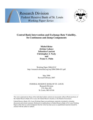
- 17. This stylized fact is supported by the timing of Reuters news collected over the 1989-1995 pe- riod.8 Although the timing of the Reuters reports should be treated cautiously, most coordinated intervention headlines fall within the overlap of the markets, suggesting that the assumption that coordinated interventions occur in the afternoon European time is reasonable. This means that, at least for the USD/EUR market, the timing of these jumps can be compared to this time range. Jumps occurring before the overlap period probably cannot be ascribed to coordinated interven- tions. Instead, such jumps might motivate intervention. But, intervention might well cause the discontinuities observed during the overlap. Intra-daily timing of jumps We first assume that coordinated interventions occur during the trading overlap of financial markets in Europe and the United States. To get a precise time for the jumps, we find the maximum intra-daily absolute exchange rate return. For both exchange rates (USD/EUR and JPY/USD), we focus on days on which there was both intervention and a discontinuity in the exchange rate. Panel 1 of Figure 5 reports the distribution of the time interval with the high- est intra-daily return for all the intervention days (coordinated or unilateral interventions) in the USD/EUR, while Panel 2 gives the same information but only for days of coordination interven- tions. Panel 2 of Figure 5 shows that for 7 out of 10 events, the maximum intra-daily exchange rate return falls within the short overlap period of U.S. and European markets. Therefore, for those 7 coordinated intervention episodes, coordinated operations might have created the jumps. Of course, other events, like macro announcements, also might have created the discontinuities. Panel 1 of Figure 5, however, also includes days of unilateral interventions. In the case of unilateral operations, the central banks can intervene over the full course of the day because there is no need to coordinate. Interestingly, the discontinuities were much more dispersed on the days of unilateral intervention. This pattern, that jumps are more concentrated on days of coordinated interventions, is consistent with the idea that intervention is related to the jumps. The same investigation might also be conducted for the interventions days on the JPY/USD market. The lack of overlap between U.S. and Japanese markets leaves the likely timing of coor- dinated intervention ambiguous, however. Nevertheless, for the sake of completeness, we provide 8Olsen and Associates provided Reuters headlines for the days of G-3 intervention from 1989 to 1995. Dominguez (2002) previously used these data for intraday analysis. 16
- 18. 0 12 24 36 48 60 72 84 96 108 120 132 144 156 168 180 192 204 216 228 240 252 264 276 288 0 1 2 3 4 Time occurrence of the maximum intra−day return − days of CBI (coordinated or unilateral) Intra−Day Periods Count of Maximum Returns Tokyo opening (0.00 GMT) Tokyo lunch starts (3.00 GMT) Tokyo lunch ends (4.30 GMT) European segment opening (6.00 GMT) North american segment opening (12.00 GMT) European segment ends (15.00 GMT) 0 12 24 36 48 60 72 84 96 108 120 132 144 156 168 180 192 204 216 228 240 252 264 276 288 0 1 2 3 4 Time occurrence of the maximum intra−day return − days of coordinated CBI Intra−Day Periods Count of Maximum Returns Tokyo opening (0.00 GMT) Tokyo lunch starts (3.00 GMT) Tokyo lunch ends (4.30 GMT) European segment opening (6.00 GMT) North american segment opening (12.00 GMT) European segment ends (15.00 GMT) Figure 5: USD/EUR - Fed and BB intervention days (Panel 1: coordinated or unilat- eral. Panel 2: coordinated) where a jump occurred. Count of daily maximum intra-day returns per intra-day periods. The graph shows, for each intra-day period, how many days have their maximum intra-day return at the intra-day interval in question. the corresponding figures for the all-type intervention days as well as the days of coordinated interventions (see Figure 6). The previous informal timing evidence can be complemented by a more robust statistical analysis of the intra-daily pattern of the exchange rate returns. The previous analysis neglects the fact that more than one jump can occur on a particular day. For instance, a second jump on the USD/EUR might occur during the overlap period, restoring the possibility that coordinated operations between the Fed and Bundesbank create this jump. Therefore, it is possible that the previous conclusion regarding the causality link for a couple of interventions is misleading. Tables 5 and 6 provide additional information with respect to the 10 CBI days where a jump occurred on the USD/EUR market, and the equivalent 14 days for the JPY/USD. For each date, we report the number of jumps we identify using the following procedure. If a day is found to contain one or more significant jumps, we neutralize the highest intra-day return (i.e. we fix it to 17
- 19. 0 12 24 36 48 60 72 84 96 108 120 132 144 156 168 180 192 204 216 228 240 252 264 276 288 0 1 2 3 4 Time occurrence of the maximum intra−day return − days of CBI (coordinated or unilateral) Intra−Day Periods Count of Maximum Returns Tokyo opening (0.00 GMT) Tokyo lunch starts (3.00 GMT) Tokyo lunch ends (4.30 GMT) European segment opening (6.00 GMT) North american segment opening (12.00 GMT) European segment ends (15.00 GMT) 0 12 24 36 48 60 72 84 96 108 120 132 144 156 168 180 192 204 216 228 240 252 264 276 288 0 1 2 3 4 Time occurrence of the maximum intra−day return − days of coordinated CBI Intra−Day Periods Count of Maximum Returns Tokyo opening (0.00 GMT) Tokyo lunch starts (3.00 GMT) Tokyo lunch ends (4.30 GMT) European segment opening (6.00 GMT) North american segment opening (12.00 GMT) European segment ends (15.00 GMT) Figure 6: JPY/USD - Fed and BoJ intervention days (Panel 1: coordinated or unilat- eral. Panel 2: coordinated) where a jump occurred). Count of daily maximum intra-day returns per intra-day periods. The graph shows, for each intra-day period, how many days have their maximum intra-day return at the intra-day interval in question. zero) and re-estimate RV and BV. We then check whether we still observe a statistically significant jump quantity. If it is the case, we reiterate the procedure all over again: we set the second highest intra-day return to zero, re-estimate the jump and so on. We do so until the BV method fails to reject the null of no jumps. This allows us to identify which discontinuities contributed to make P κ2 a statistically significant quantity.9 Tables 5 and 6 provide the number of significant jumps, the timing of the three highest intra-daily returns, the magnitude of P κ2 and its ranking in the global unconditional sample. Table 5 suggests that two of the three intervention days, for which the highest intra-daily return occurred before the overlap period, had more than one significant jump. For these two 9We must admit that our procedure to count the number of significant jumps in the day is ad hoc and unlikely to be fully rigorous. Monte Carlo simulations with a jump-diffusion GARCH model imply, however, that our method is fairly accurate with fewer than 10 jumps (discontinuities) per day. Therefore we believe it provides useful information that would otherwise be unavailable with bipower variation. 18
- 20. Date # jumps Max #1 time Max #2 time Max #3 time P κ2 Global rank 1987-12-10 1 13.40 - - 1.753219 8 1988-04-14 2 12.40 12.45 - 0.585892 31 1988-09-26 1 13.10 - - 0.066267 383 1989-02-03 1 14.35 - - 0.394049 59 1989-10-05 1 13.05 - - 0.330991 70 1991-02-12 10 9.50 15.40 8.45 0.083371 340 1991-03-11 1 9.35 - - 0.218730 122 1992-08-11 1 12.20 - - 0.299545 77 1992-08-21 1 13.25 - - 0.460832 46 2000-09-22 2 11.15 12.05 - 7.108620 1 Table 5: USD/EUR - 10 days where a coordinated intervention occurred and a dis- continuity ( P κ2 ) is detected. For each date, we provide the number of jumps (# jumps), the time at which the three greatest intra-day returns occurred, the magnitude of the detected jump ( P κ2 ) and its rank in the global jump ranking (in the unconditional sample). days (February 12, 1991 and September 22, 2000), coordinated interventions during overlap period might have created the second jump, which occurred during the overlap period. For only one of the 10 days of coordinated interventions (March 11, 1991), there was no significant jump during the overlap, which suggests that coordinated intervention was less likely to produce the jump. The assumption that coordinated interventions take place only during the overlap is supported by only tenuous evidence. Coordinated interventions might occur before or after the overlap period, suggesting that some other type of information should be used. One possibility is to use the timing of the Reuters reports of interventions for the 10 days for which jumps and interventions were detected on the USD/EUR market. Nevertheless, the timing of these news reports is available only between 1989 and 1995. Before 1989, we infer timing of intervention from the level of exchange rate at which the reported intervention took place, obtained from news reports. Since it is likely that over the full course of the trading day this exchange rate level will be crossed several times, there are several possible timings for this report. We also must disregard the days for which multiple jumps were detected, such as December 12, 1992. All in all, we scrutinize 4 occurrences to infer the nature of the causal relationship between jumps and interventions. Table 7 reports the date, the timing of the first jump and the timing of the Reuters news for 19
- 21. Date # jumps Max #1 time Max #2 time Max #3 time P κ2 Global rank 1987-04-10 2 12.35 0.10 - 0.310725 102 1987-04-24 1 3.35 - - 0.312094 101 1987-11-30 1 0.05 - - 0.086187 421 1988-04-14 1 12.45 - - 0.424126 51 1988-10-31 3 14.25 8.00 16.20 0.122487 316 1989-09-29 1 0.15 - - 0.236308 140 1989-10-05 1 13.20 - - 0.337824 85 1989-11-20 1 16.45 - - 0.040149 553 1990-01-18 1 13.40 - - 0.043575 544 1992-02-18 5 9.35 8.10 0.40 0.196976 181 1994-05-04 1 12.30 - - 0.283198 114 1994-11-02 1 16.05 - - 0.454362 42 1995-04-03 1 23.55 - - 0.631489 23 1995-07-07 11 15.20 12.50 13.40 0.247987 132 Table 6: JPY/USD - 14 days where a coordinated intervention occurred and a jump ( P κ2 ) is detected. For each date, we provide the number of jumps (# jumps), the time at which the three greatest intra-day returns occurred, the magnitude of the detected jump ( P κ2 ) and its rank in the global jump ranking (in the unconditional sample). Date Timing of first jump Timing of first report 1989-10-05 13.05 12.10 1991-03-11 9.35 9.45 1992-08-11 12.20 12.23 1992-08-21 13.25 13.34 Table 7: Dollar/Euro - 4 days where a coordinated intervention occurred and one discontinuity ( P κ2 ) is detected. For each date, we provide the date, the timing of the first jump and the timing of the Reuters news. these 4 days. For one day, the report of intervention precedes the jump, suggesting that interven- tion did not react to this jump. For the three other days, the first report of intervention occurs shortly after (within 10 minutes of) the jump. The fact that the reports of intervention follow 20
- 22. the maximal return so very closely indicates that the intervention is likely to have preceded the jump and caused it, rather than the other way around. We believe that the timing evidence is consistent with intervention preceding/causing jumps because CBs need time to detect the jump, to react and to implement the currency orders. It is difficult to imagine that a CB is able to react in less than 3 minutes to the occurrence of jumps. Further, there is a lag between intervention and the time it is reported on the newswire, as documented by Fischer (2005). We believe that the most plausible interpretation is that intervention preceded and caused the jumps, but was reported after. We find it somewhat less plausible, but possible, that intervention created jumps that were used by traders to detect intervention (and to report the CB’s presence in the market). This story is supported by some evidence provided by Gnabo, Laurent, and Lecourt (2006) for the yen/dollar market. While it is again difficult to formally check this sequence of events with the current dataset, the evidence provided here tends to refute a causal relationship running from jumps to interventions. Of course, given the very small sample, further investigation should be conducted to examine the possibility of reverse causation, i.e. interventions creating jumps. Jump sign and intervention direction This section has shown a relation between jump size and coordinated intervention. Days of intervention tend to have unusually large jumps (see Table 4) and jumps tend to occur dispropor- tionately during the same hours that U.S. and Buba intervention is said to take place (See Figure 5). The direction of causality, if any, remains diputable, however. It is possible that intervention either reacts to jumps or that intervention causes jumps. We have one final procedure to attempt to determine the likely direction of causality. We can examine the direction of the interventions and jumps to see if one can informally infer the direction of causality. If purchases of USD are associated with a jump decline in the value of the USD, that would imply that the central bank reacted to the jump by leaning against the wind. The alternative inference-that intervention creates a very sharp perverse movement in the exchange rate-is very implausible. On the other hand, if purchases of USD are associated with a jump upward in the value of the USD, that would tend to imply that the intervention caused the jump in the exchange rate. Although one cannot categorically rule out the possibility the central banks lean with the jumps, it seems much less likely. What does the direction of intervention/jumps tell us about causality? Table 8 shows the dates of jumps and coordinated interventions for the USD/EUR (top panel) and the JPY/USD 21
- 23. (bottom panel). The columns of the table show the date, the maximal intraday returns and the sign of the intervention (buy or sell USD). For 8 of the 10 observations of the USD/EUR, the data are consistent with intervention causing the jumps. That is, in 8 of the 10 cases, a buy (sale) of USD through intervention was associated with a negative (positive) maximal intraday return in USD/EUR. The two days which do not fit this pattern occurred during the ”Louvre period,” during which the major aim of central banks was to smooth volatility, so they were likely to react strongly to jumps. Similarly, for the JPY/USD, in 12 of 14 cases, a buy (sale) of USD was associated with a positive (negative) return to the JPY/USD. 10 Therefore we conclude that an examination of the direction of intervention and jumps is consistent with interventions normally causing jumps, rather than the other way around. Macro news announcements Several empirical studies have documented that macroeconomic announcements can generate jumps in the exchange rates (Andersen, Bollerslev, Diebold, and Vega 2003, Barndorff-Nielsen and Shephard 2006). These scheduled announcements can induce large swings in the value of the cur- rencies, especially when the announced value deviates from the market’s expectation. Therefore, it is important to control for the occurrence of macroeconomic news to isolate the subset of the jumps that could be attributed to CBIs. Table 9 lists the major types of macroeconomic announcements that can be considered as ‘control variables’ in our analysis. The table provides details about the days on which the news is released, the units of measurement and the available sample. Using the data about these macro announcements, we can focus on the days of coordinated interventions. In particular, we can identify on which days major macroeconomic announcements occurred. While it might be difficult to identify which type of news tends to impact the behavior of FX traders and the value of the exchange rates, we can pay some particular attention to news concerning the trade balance as well as the U.S. exports and imports. Table 10 identifies which macro announcement occurred on days of coordinated interventions where a jump was detected. We provide the rank of the surprise in the ranking of surprises in absolute value and , in parenthesis, the magnitude of surprises (in standard deviation). It shows that half of the intervention days for which we found jumps on the JPY/USD were also days on 10Note that the exchange rates are quoted differently, so a rise in the USD/EUR means a depreciation of the USD but a rise in the JPY/USD means an appreciation of the USD. 22
- 24. Table 8: For dates of jump and coordinated interventions on the USD/EUR (upper panel) and JPY/USD (lower panel) markets, we match the magnitude of jump returns with the direction of interventions (buy or sell USD). Note that a rise in the USD/EUR means a depreciation of the dollar and a rise in the JPY/USD means an appreciation of the dollar. Date Max n1 Max n2 Max n3 Intervention sign USD/EUR 1987-12-10 1.392788 - - buy 1988-04-14 0.646169 0.642020 - buy 1988-09-26 0.178459 - - sell 1989-02-03 0.571180 - - sell 1989-10-05 0.475811 - - sell 1991-02-12 -0.171818 0.171641 -0.158588 buy 1991-03-11 0.348711 - - sell 1992-08-11 -0.643359 - - buy 1992-08-21 -0.602769 - - buy 2000-09-22 2.788306 0.973860 - sell JPY/USD 1987-04-10 0.317013 -0.278843 - buy 1987-04-24 0.483136 - - buy 1987-11-30 -0.165838 - - buy 1988-04-14 -0.540055 - - buy 1988-10-31 0.236184 0.224072 0.199243 buy 1989-09-29 -0.345301 - - sell 1989-10-05 -0.340885 - - sell 1989-11-20 -0.152318 - - sell 1990-01-18 -0.130084 - - sell 1992-02-18 0.312745 0.282475 -0.177148 buy 1994-05-04 0.486739 - - buy 1994-11-02 0.719446 - - buy 1995-04-03 0.834898 - - buy 1995-07-07 0.310470 0.231750 0.231080 buy 23
- 25. Announcement Variable Name Range freq Unit Day of the week Labor market Unemployment Rate UNEMPLOY 1986-2005 m %rate Usually Friday Employees on Payrolls NFPAYROL 1986-2005 m change in 1000 Usually Friday Prices Producer Price Index PPI 1986-2005 m %change Tuesday to Friday Consumer Price Index CPI 1986-2005 m %change Tuesday to Friday Business cycle conditions Durable Good Orders DURABLE 1986-2005 m %change Tuesday to Friday Housing Starts HOUSING 1986-2005 m millions Tuesday to Friday Leading Indicators LEADINGI 1986-2005 m %change Monday to Friday Trade Balance TRADEBAL 1986-2005 m $ billion Tuesday to Friday U.S. Exports USX 1986-2005 m $ billion Tuesday to Friday U.S. Imports USI 1986-2005 m $ billion Tuesday to Friday Table 9: Set of available macro announcements 24
- 27. which macroeconomic announcements were made. There is nevertheless only one day (April 14, 1988) for which some news regarding the trade balance and U.S. trade flows was released. The timing of the jump on this day is around 12.45 GMT. Turning to the USD/EUR, we identify 3 days of coordinated interventions for which macro announcements occurred. Interestingly, we found also April 14, 1988 as one of these days and the timing of the jump identified for the USD/EUR and JPY/USD are almost the same. On December 10, 1987, the trade balance news was released at 13:30 GMT and the identified jump occurs around 13.40 GMT. It seems very likely that the trade balance announcement generated the jump for this day. In summary, it appears that major macroeconomic announcements did not generate all of the jumps identified on the days of coordinated interventions. Instead, coordinated intervention might have caused some of these discontinuities. Nevertheless, one should keep in mind that this sample is very small, less that 10% of the coordinated interventions. A related question is whether coordinated interventions impact the continuous component of realized volatility. The next section examines this issue. 4.3 Regression analysis Up to now, we have investigated the relationship between CBIs and the jump component of the RV. In seems that CBIs create only a small number of jumps. For instance, out of the 106 coordinated interventions of the Fed and the Bundesbank, only 7 or 8 interventions seem to have induced some jumps on the exchange rate. Although intervention does not create many jumps, the intraday data do seem to strongly suggest that some coordinated interventions are very closely related to jumps and are plausibly the cause of those few jumps. Most of the previous empirical studies of the impact of CBIs on exchange rate volatility find that CBIs tend to increase exchange rate volatility (see Humpage, 2003 for a recent survey). In particular, Dominguez (2004) and Beine, Laurent, and Palm (2005) find that intervention has a strong and robust impact on the realized volatility of the major exchange rates. The latter paper found that this result holds for concerted interventions, with impact lasting for a couple of hours. The analysis was carried out using hourly intra-daily returns for the EUR/USD market and focused on the period ranging from 1989 to 2001. There is disagreement, however, about whether intervention causes higher volatility, or simply reacts to it. Neely (2005a), for example, argues that the finding that intervention causes higher volatility is likely due to improper identification of the structural parameters. 26
- 28. We first extend the analysis of the relation of volatility and intervention by regressing log(RVt) computed at 21.00 GMT on the dummies capturing days of interventions as well as a set of day- of-the-week dummies to capture intra-weekly variation in the volatility of exchange rates.11 In contrast to Beine, Laurent, and Palm (2005), the estimates of realized volatility are built from 5-minute intra-daily returns. Due to the fact that these estimates of daily volatility include the 288 previous squared returns, the impact of the interventions should be captured by the daily estimates of volatility even though this impact displays a low degree of persistence. More formally, we allow for long memory in the volatility process and, following Andersen, Bollerslev, Diebold, and Labys (1999), estimate several specifications of the following ARFIMA(1, d, 0) model: (1 − φL)(1 − L)d £ log(σ2 t ) − µ ¤ = ²t + αt + νt + µt, (18) where σ2 t is the daily realized volatility or its continuous component, and d (the fractional inte- gration parameter), φ, µ are parameters to be estimated. We control for day-of-the-week seasonal effects through αt αt = α1MONDAYt + α2TUESDAYt + α3WEDNESDAYt + α4THURSDAYt, (19) where MONDAYt, TUESDAYt, WEDNESDAYt, and THURSDAYt are day-of-the-week dum- mies and for macro announcements effects through νt νt =θ1CPIt + θ2DURABLEt + θ3HOUSINGt + θ4LEADINGIt (20) + θ5NFPAY ROLt + θ6PPIt + θ7TRADEBALt + θ8UNEMPLOYt, where α1 to α4 and θ1 to θ8 are additional parameters to estimate. The macro announcements variables are the absolute value of the surprise component of the corresponding macro announce- ments described in Section 4.2. Though we control for these variables, we do not report the estimates because that falls beyond the scope of this paper. Moreover, we present results for two different specifications of µt. First, µt includes binary variable for unilateral and coordinated interventions of central banks on their respective markets 11The extension of the investigation period is not trivial in the sense that it leads to a big increase in the number of days of coordinated and unilateral interventions. Indeed, while we observed 58 coordinated interventions over the 1989-2001 period, the inclusion of 1987 and 1988 leads to the inclusion of 48 additional coordinated interventions. This might be explained by the fact that this period belongs to the so-called post-Louvre agreement period, during which concerted operations were conducted in order to get rid of excessive exchange rate volatility. 27
- 29. (i.e. we consider effects of Fed and Bundesbank interventions, unilateral and coordinated, on the USD/EUR, and Fed and BoJ interventions, unilateral and coordinated, on the JPY/USD): USD/EUR: µt = β1BBUt + β2FEDUt + γCOORDt, (21) JPY/USD: µt = β1BOJUYt + β2FEDUYt + γCOORDYt, (22) where β’s and γ are parameters to be estimated. BBUt, FEDUt, and COORDt are dummies for unilateral Bundesbank interventions, unilateral Fed interventions, and coordinated Bundesbank- Fed interventions on the USD/EUR market, respectively. BOJUYt, FEDUYt, and COORDYt are, mutatis mutandis, the corresponding dummies for unilateral BoJ interventions, unilateral Fed interventions, and coordinated BoJ-Fed interventions on the JPY/USD market. Secondly, we look for a different relation of volatility with coordinated interventions on days with and without significant jumps (α = 0.9999). The variables COORDt and COORDYt are thus split into two parts: COORDJ and COORDY J for coordinated interventions on jump days, and COORDNOJ and COORDY NOJ for coordinated interventions on days where no jumps were detected. We then have the following specifications for µt: USD/EUR: µt = β1BBUt + β2FEDUt + δ1COORDJt + δ2COORDNOJt, (23) JPY/USD: µt = β1BOJUYt + β2FEDUYt + δ1COORDY Jt + δ2COORDY NOJt, (24) where δ’s are additional parameters to estimate. The results for the USD/EUR, reported in the left panel of Table 11, suggest that both uni- lateral interventions and coordinated interventions of the Fed and the BB tend to be associated with higher exchange rate volatility (second column labeled ‘log(RV )’). This is especially obvious for coordinated interventions, which have an even stronger association with volatility, compared with those associated to unilateral operations. The column labeled ‘log(C)’ in Table 11 reports the same results for the log of the continuous part of realized volatility as described in Equation (15). These results suggest that this component was related to intervention. The magnitude of the coefficients, and their significance, are quite similar between the second and third columns. This suggests that CBIs explain, in a statistical sense, volatility. The last two columns of each panel of Table 11 report the same results obtained from regressing the log of realized volatility and the log of the continuous component on the intervention dummies. In contrast to the previous regressions, the specification accounts for a break down of coordinated 28
- 31. interventions between those found associated with the jumps (denoted COORDJ in the Tables, 10 occurrences) and the remaining ones (denoted COORDNOJ, 96 occurrences). Coordinated interventions that are potentially associated with jumps have a strong correlation with realized volatility but a weaker association with continuous volatility (see the coefficients labeled δ1 (CO- ORDJ/COORDYJ). This confirms the previous findings that when CBIs are associated with a jump, the size of the jump is higher and thus the association with realized volatility is substantial. Coordinated interventions associated with jumps also have some impact on the continuous part. The right panel of Table 11 presents the same results for the JPY/USD. Reassuringly, the results are consistent with those obtained for the USD/EUR. To sum up, we found clear relation between coordinated interventions, realized volatility and its continuous component. Interventions associated with jumps display a bigger correlation with realized volatility and still have a relation with continuous volatility. 5 Interpretation of the findings and significance for central bank foreign exchange market policy The empirical findings of this paper show that realized volatility of exchange rates between major currencies is driven by a persistent continuous component and a jump component. The method of bipower variation permitted us to decompose realized volatility into these two components (see Barndorff-Nielsen and Shephard, 2004, 2006, and Andersen, Bollerslev, and Diebold, 2005). The findings indicate that the jump component is important in the major foreign exchange markets. Both macroeconomic announcements and coordinated interventions generate jumps. A more extended study of the factors that explain the occurrence of jumps would be interesting and relevant from a scientific point of view, as well as being potentially useful for hedging applications. On the whole, the findings confirm that CBIs are associated with increased exchange rate volatility.12 Furthermore, there is some evidence that interventions tend to create jumps in the exchange rate volatility. Intervention does not cause many jumps, but jumps associated with interventions tend to be larger than normal. As a result, CBIs tend, on average, to be associated with high exchange rate volatility. Interventions are associated with the continuous part of the volatility process as well. This is confirmed by the regression analysis, in particular by the striking similarity between the results for realized volatility, as a dependent variable, and for the continuous 12See e.g. Beine, Laurent, and Palm (2005), Dominguez (1998) and Dominguez (2003). 30
- 32. component of exchange rate volatility. The method for decomposing realized volatility into two components yields approximate results. There may be a remaining part of the jump left in the continuous component. If interventions had in fact been aimed at attenuating or eliminating jumps only, the finding that CBIs affect the continuous part could be due to an approximation error in the decomposition. From the analysis of the timing of the occurrence of jumps there is much less evidence that the central banks react to jumps in foreign exchange rates. This finding indicates that the causation is mostly unidirectional in the sense that coordinated interventions by central banks affect jumps. But interventions sometimes appear to produce significant discontinuities and are associated with a higher persistent continuous component of realized volatility. Allowing for differences in the impact (δi) of interventions between days on which jumps occurred and days without jumps, a likelihood ratio test concludes that the δi’s significantly differ for log(RV ) for the USD/EUR but do not significantly differ form each other for log(C). For the JPY/USD, the δi’s do not significantly differ from each other for log(RV ) and for log(C). These findings suggests that, on both markets, coordinated CBIs had the same positive association with the persistent part of realized volatility whether the market was prone to jumps or not. On the USD/EUR market, coordinated CBIs seem to create jumps that are more than three times as large as those observed on other days. Finally, it is worthwhile to note that unilateral interventions by the Federal Reserve Bank and by the Bank of Japan are significantly positively associated with realized volatility and its continuous component. Unilateral interventions by the European Central Bank in the USD/EUR market are associated with higher volatility, but not to a statistically significant degree. These results have been obtained while accounting for macroeconomic announcements, such as the un- employment rate, the number of employees on payroll, the producer and consumer price index, the durable goods order, the housing starts, the leading indicators and the trade balance. The finding of a positive association of CBIs with market volatility is consistent with pre- dictions from both the inventory-based approach and the information-based approaches in the microstructure literature. The inventory-based approach (see e.g. O’Hara, 1995, and Lyons, 2001) emphasizes the balancing problem on foreign exchange markets resulting from (stochastic) inflow and outflow deviations. Such deviations could result from a policy intervention. Theory predicts that these deviations will be temporary and last until portfolios have been rebalanced. The information-based approach focuses on the process of learning and price formation on markets. 31
- 33. In high volatility periods, much trading can take place as informed traders can easily hide the vol- ume of their transactions. This approach predicts an increase in transactions volume and volatility following a CBI. Once the intervention news has been revealed, transaction volume, prices and volatility should revert to their pre-intervention levels. Longer-run effects are related to factors such as information processing. Turbulent market conditions might require more time to revert to their initial levels. Our findings are in line with both theoretical explanations. One should nev- ertheless realize that both approaches provide little insight into how long-run adjustment takes place. 6 Conclusion This paper has studied the relation between intervention and the continuous and discontinuous (jump) components of exchange rate volatility in the USD/EUR and the JPY/USD markets. Our study focuses on days in which there is both coordinated intervention and jumps. Intervention is not associated with an increased likelihood of jumps at the daily frequency. It is, however, associated with much larger jumps than normal. Analysis of the timing and direction of discontinuities and CBIs strongly suggests that interventions normally cause jumps, rather than reacting to them. The period of the Louvre Accord-during which central banks tried particularly hard to dampen volatility-provided a couple of exceptions to that rule. In that period, intervention did seem to react to jumps by leaning against the wind. These results are robust to the inclusion of macro economic announcements in the analysis. Coordinated CBIs were found to be significantly associated with both higher realized volatility and its continuous component. The reduced form relationship between coordinated intervention and volatility is even stronger on days with jumps. The main finding that interventions are associated with higher exchange rate volatility is consistent with previous empirical studies and with predictions from the theoretical literature on the inventory-based and the information based approaches. Before drawing strong conclusions about possible unintended adverse effects of CBIs on volatil- ity in foreign exchange markets it would be sensible to study more deeply the caution issue. Ques- tions which require more attention are for instance: Do central bank have inside information allow- ing them to predict turbulences and act on them on short notice? Would the turbulences/jumps in volatility have been more severe if central banks had not intervened? Do the jumps-apparently caused by intervention-tend to move the exchange rate toward longer run fundamental values, 32
- 34. away from those values or are they just noise? What is the role of macroeconomic announcements in generating turbulences on foreign exchange markets? 33
- 35. References Andersen, T. G., and T. Bollerslev (1998a): “Answering the Skeptics: Yes, Standard Volatil- ity Models do Provide Accurate Forecasts,” International Economic Review, 39, 885–905. (1998b): “DM-Dollar Volatility: Intraday Activity Patterns, Macroeconomic Announce- ments and Longer Run Dependencies,” The Journal of Finance, 53, 219–265. Andersen, T. G., T. Bollerslev, and F. X. Diebold (2005): “Roughing It Up: Including Jump Components in the Measurement, Modeling and Forecasting of Return Volatility,” NBER Working Paper 11775, forthcoming in Review of Economics and Statistics. Andersen, T. G., T. Bollerslev, F. X. Diebold, and P. Labys (1999): “Realized Volatility and Correlation,” L.N. Stern School of Finance Department Working Paper 24. (2001): “The Distribution of Realized Exchange Rate Volatility,” Journal of the American Statistical Association, 96, 42–55. Andersen, T. G., T. Bollerslev, F. X. Diebold, and C. Vega (2003): “Micro Effects of Macro Announcements: Real-Time Price Discovery in Foreign Exchange,” The American Economic Review, 93, 38–62. Baillie, R. T., and W. P. Osterberg (1997): “Why do Central Banks Intervene ?,” Journal of International Money and Finance, 16, 909–919. Barndorff-Nielsen, O., J. Graversen, J. Jacod, M. Podolskij, and N. Shephard (2005): “A central Limit Theorem for Realized Power and Bipower Variation of Continuous Semimartingale,” in From Stochastic Analysis to Mathematival Finance, Festschrift for Albert Shiryaev, ed. by Y. Kabanov, and R. Lipster. Springer Verlag. Barndorff-Nielsen, O., and N. Shephard (2002a): “Econometric Analysis of Realised Volatility and its use in Estimating Stochastic Volatility Models,” Journal of the Royal Sta- tistical Society, 64, 253–280. (2002b): “Estimating Quadratic Variation Using Realized Variance,” Journal of Applied Econometrics, 17, 457–478. (2004): “Power and Bipower Variation with Stochastic Volatility and Jumps (with Dis- cussion),” Journal of Financial Econometrics, 2, 1–48. 34
- 36. (2006): “Econometrics of Testing for Jumps in Financial Economics Using Bipower Variation,” Journal of Financial Econometrics, 4, 1–30. Beine, M., A. Bénassy-Quéré, and C. Lecourt (2002): “Central Bank Intervention and Foreign Exchange Rates: New Evidence from FIGARCH Estimations,” Journal of International Money and Finance, 21, 115–144. Beine, M., S. Laurent, and F. Palm (2005): “Central Bank Forex Interventions Assessed Using Realized Moments,” Working Paper. Bonser-Neal, C., and G. Tanner (1996): “Central Bank Intervention and the Volatility of Foreign Exchange Rates: Evidence from the Options Market,” Journal of International Money and Finance, 15, 853–878. Catte, P., G. Galli, and S. Rebecchini (1992): “Exchange Markets Can Be Managed!,” Report on the G-7, International Economic Insights. Comte, F., and E. Renault (1998): “Long Memory in Continuous Time Stochastic Volatility Models,” Mathematical Finance, 8, 291–323. Dominguez, K. M. (1998): “Central Bank Intervention and Exchange Rate Volatility,” Journal of International Money and Finance, 17, 161–190. (2003): “The Market Microstructure of Central Bank Intervention,” Journal of Interna- tional Economics, 59, 25–45. (2004): “When Do Central Bank Interventions Influence Intra-daily and Longer-Term Exchange Rate Movements,” Forthcoming in Journal of Financial Economics. Fischer, A., and M. Zurlinden (1999): “Exchange Rate Effects of Central Bank Interventions: An Analysis of Transaction Prices,” Economic Journal, 109, 662–676. Fischer, Andreas, M. (2005): “On the Inadequacy of Newswire Reports for Empirical Research On Foreign Exchange Interventions,” Swiss National Bank Working Papers 2005-2. Galati, G., and W. Melick (1999): “Central Bank Intervention and Market Expectations: an Empirical Study of the YEN/Dollar Exchange Rate, 1993-1996,” BIS Working Paper 77. 35
- 37. Gnabo, J., S. Laurent, and C. Lecourt (2006): “Does Transparency in Central Bank Inter- vention Policy Bring Noise in the Market? The Case of the Bank of Japan,” mimeo, University of Namur. Huang, X., and G. Tauchen (2005): “The Relative Contribution of Jumps to Total Price Variation,” Journal of Financial Econometrics, 3, 456–499. Humpage, O. F. (2003): “Government Intervention in the Foreign Exchange Market,” Federal Reserve Bank of Cleveland, Working Paper 03-15. Kearns, J., and R. Rigobon (2004): “Identifying the Efficacy of Central Bank Interventions: Evidence from Australia and Japan,” Forthcoming in Journal of International Economics. Lyons, R. K. (2001): The Microstructure Approach to Exchange Rates. The MIT Press, Cam- bridge, MA. Neely, C. J. (2000): “The Practice of Central Bank Intervention: Looking Under the Hood,” Federal Reserve Bank Working Paper no. 2000-028. (2005a): “An Analysis of Recent Studies of the Effect of Foreign Exchange Intervention,” Federal Reserve Bank of Saint Louis, Working Paper no. 2005-03B. (2005b): “Identifying the Effect of US Interventions on the Level of Exchange Rates,” Federal Reserve Bank of Saint Louis, Working Paper no. 2005-031B. O’Hara (1995): Market Microstructure Theory. Basic Blackwell, Basic Blackwell. 36