5. 2-dimensional square lattice
Order
• Spatial
• Dimensional
Spatial : depending on the extent in space (length scale) up to which the 3-dimensional
order persists Eg: crystal (millimeters or above)
Dimensional : depending on the number of dimensions in which long range order persists
Eg: crystal (typically 3-dimension)
Order implies predictability of atom/molecule position and molecule orientation
10. Point group symmetries :
Identity (E)
Reflection (s)
Rotation (Rn)
Rotation-reflection (Sn)
Inversion (i)
In periodic crystal lattice :
(i) Additional symmetry - Translation
(ii) Rotations – limited values of n
11. Restriction on n-fold rotation symmetry
in a periodic lattice
a
a
na
q
(n-1)a/2
cos (180-q) = - cos q = (n-1)/2
n 3 2 1 0 -1
qo 180 120 90 60 0
Rotation 2 3 4 6 1
Possible values of n with the condition
12. Crystal Systems in 2-dimensions - 4
square
rectangular
oblique
hexagonal
13. Oblique a b, 90o
Rectangular a b, = 90o
Square a = b, = 90o
Hexagonal a = b, = 120o
15. In geometry and crystallography, a Bravais lattice is a category of translative
symmetry groups (also known as lattices) in three directions.
Such symmetry groups consist of translations by vectors of the form
R = n1a1 + n2a2 + n3a3,
where n1, n2, and n3 are integers and a1, a2, and a3 are three non-coplanar vectors,
called primitive vectors.
16. Bravais lattices in 2-dimensions - 5
square rectangular
oblique hexagonal
centred rectangular
The Bravais lattices were studied by Moritz Ludwig Frankenheim in 1842, who found
that there were 15 Bravais lattices in 3D crystals. This was corrected to 14 by A. Bravais
in 1848.
17. Primitive cube (P)
Bravais Lattices in 3-dimensions
(in cubic system)
Body centred cube (I)
Face centred cube (F)
18. Bravais Lattices in 3-dimensions - 14
Cubic - P, F (fcc), I (bcc)
Tetragonal - P, I
Orthorhombic - P, C, I, F
Monoclinic - P, C
Triclinic - P
Trigonal - R
Hexagonal/Trigonal - P
There are seven different kinds of lattice systems, and each kind of lattice system has
four different kinds of centering (primitive, base-centered, body-centered, face-
centered). However, not all of the combinations are unique; some of the combinations
are equivalent while other combinations are not possible due to symmetry reasons.
This reduces the number of unique lattices to the 14 Bravais lattices.
21. Every point in a Bravais lattice has identical environment; observation from any
point is identical. This aspect can be used to distinguish a non-Bravais lattice from
a Bravais lattice
For example, a honeycomb lattice is not a Bravais lattice, as the points shown in colour dots
do not have identical environment; however, combination of two of these points leads to the
hexagonal Bravais lattice in 2-D.
22. Lattice (o)
X X X X X X X X
X X X X X X X X
X
X
X X X X X X X X
X X X X X X X X
X
X
X X X X X X X X
X X X X X X X X
X
X
X X X X X X X X
X X X X X X X X
X
X
X X X X X X X X X
+ basis (x) = crystal structure
‘lattice’ is a set of points in space described by a set of coordinates, two in 2-D or three in 3-D.
The object or set of objects placed on the lattice points, is described technically as the ‘basis
A crystal consists of the basis organized on a lattice with a specified symmetry
24. Lattice +
Nonspherical Basis
Point group
operations
Point group
operations +
translation
symmetries
7 Crystal systems 32 Crystallographic
point groups
14 Bravais lattices 230 space groups
Lattice +
Spherical Basis
Space Groups
25. x
y
z
(100)
Miller plane
Distance
between
planes = a
a
Miller Indices are a method of describing the orientation of a plane or set of planes within
a lattice in relation to the unit cell. They were developed by William Hallowes Miller.
26. These indices are useful in understanding many phenomena in materials science,
such as explaining the shapes of single crystals, the form of some materials'
microstructure, the interpretation of X-ray diffraction patterns, and the movement of a
dislocation, which may determine the mechanical properties of the material.
27.
28.
29.
30.
31.
32.
33.
34.
35.
36.
37.
38. Lattice planes can be represented by showing the trace of the planes on the
faces of one or more unit cells. The diagram shows the trace of the
planes on a cubic unit cell.
39.
40.
41.
42.
43. Vectors and Planes
It may seem, after considering cubic systems, that
any lattice plane (hkl) has a normal direction [hkl].
This is not always the case, as directions in a crystal
are written in terms of the lattice vectors, which are
not necessarily orthogonal, or of the same magnitude.
A simple example is the case of in the (100) plane of
a hexagonal system, where the direction [100] is
actually at 120° (or 60° ) to the plane. The normal to
the (100) plane in this case is [210]
48. Time Line
• 1665: Diffraction effects observed by Italian
mathematician Francesco Maria Grimaldi
• 1868: X-rays Discovered by German Scientist
Röntgen
• 1912: Discovery of X-ray Diffraction by Crystals:
von Laue
• 1912: Bragg’s Discovery
52. X-ray Spectra
• Continuous spectra (white radiation)–
range of X-ray wavelengths generated by
the absorption (stopping) of electrons by
the target
• Characteristic X-rays – particular
wavelengths created by dislodgement of
inner shell electrons of the target metal;
x-rays generated when outer shell
electrons collapse into vacant inner
shells
• K peaks created by collapse from L to K
shell;
K peaks created by collapse from M to
K shell
K
K
X
When light hits an electron, the
electron jumps to a higher energy
level, then drops back to its original,
shell, emitting light
57. q
dhkl
hkl plane
2dhkl sinq = nl
q
Wavelength = l
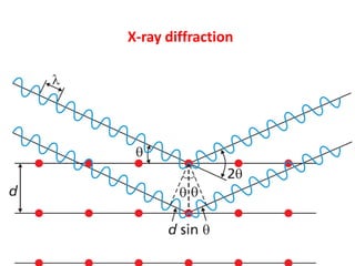
Bragg’s law
• Diffraction from a three dimensional periodic structure such as atoms in a
crystal is called Bragg Diffraction.
• Similar to diffraction though grating.
• Consequence of interference between waves reflecting from different
crystal planes.
• Constructive interference is given by Bragg's law:
• Where λ is the wavelength, d is the distance between crystal planes, θ is
the angle of the diffracted wave. and n is an integer known as the order of
the diffracted beam.
67. von Laue’s condition for x-ray diffraction
d
k k
lattice point
k = incident x-ray wave vector
k = scattered x-ray wave vector
d = lattice vector
d.i -d.i
i = unit vector = (l/2)k
i = unit vector = (l/2)k
Constructive interference condition:
d.(i-i) = ml
(l/2)d.(k-k) = ml
d.k = 2m
K = reciprocal lattice vector
d.K = 2n
k = K
Can be recast in the
language of wave vectors
and translations in
momentum space
(reciprocal lattice space)
obtained by the Fourier
transform of the periodic
real lattice space.
https://www.youtube.com/watch?v=JY3sALtySBk
68.
69. Real space Reciprocal space
Crystal Lattice Reciprocal Lattice
Crystal structure Diffraction pattern
Unit cell content Structure factor
x
y
y’
x’
y’
x’
70. Fhkl = S fn e2i(hx +ky +lz )
n n n
Relates to
Atom type
Atom position
Structure factor
Intensity of x-ray scattered from an
(hkl) plane
Ihkl Fhkl
2
71. Structure Factor
2 ( )
1
n n n
N
i hu kv lw
hkl n
F f e
− h,k,l : indices of the diffraction plane under consideration
− u,v,w : co-ordinates of the atoms in the lattice
− N : number of atoms
− fn : scattering factor of a particular type of atom
Bravais Lattice Reflections possibly present Reflections necessarily absent
Simple All None
Body Centered (h+k+l): Even (h+k+l): Odd
Face Centered h, k, and l unmixed i.e. all
odd or all even
h, k, and l: mixed
Intensity of the diffracted beam |F|2
75. Reciprocal lattice vectors
Used to describe Fourier analysis of electron
concentration of the diffracted pattern.
Every crystal has associated with it a crystal lattice and
a reciprocal lattice.
A diffraction pattern of a crystal is the map of reciprocal
lattice of the crystal.
99. Diffraction from a variety of materials
(From “Elements of X-ray
Diffraction”, B.D. Cullity,
Addison Wesley)
100. Effect of particle size on diffraction lines
2q 2q
B
Amax
½Amax
2qB (Bragg angle) 2qB
Particle size small Particle size large
2q1 2q2
101. Scherrer formula for particle size estimation
t =
0.9l
B cosqB
t = average particle size
l = wavelength of x-ray
B = width (in radians) at half-height
qB = Bragg angle
102.
103.
104.
105.
106.
107. Indexing to other Crystal Systems
Tetragonal: 1/dhkl
2 = (h2+k2)/a2 + l2/c2
Orthorhombic: 1/dhkl
2 = h2/a2 + k2/b2 + l2/c2
Hexagonal: 1/dhkl
2 = 4(h2+k2+hk)/3a2 + l2/c2
108. Analysis of Single Phase
Intensity
(a.u.)
2q(˚) d (Å) (I/I1)*100
27.42 3.25 10
31.70 2.82 100
45.54 1.99 60
53.55 1.71 5
56.40 1.63 30
65.70 1.42 20
76.08 1.25 30
84.11 1.15 30
89.94 1.09 5
I1: Intensity of the strongest peak
109. Procedure
• Note first three strongest peaks at d1, d2, and d3
• In the present case: d1: 2.82; d2: 1.99 and d3: 1.63 Å
• Search JCPDS manual to find the d group belonging to the strongest
line: between 2.84-2.80 Å
• There are 17 substances with approximately similar d2 but only 4 have
d1: 2.82 Å
• Out of these, only NaCl has d3: 1.63 Å
• It is NaCl……………Hurrah
Specimen and Intensities Substance File Number
2.829 1.999 2.26x 1.619 1.519 1.499 3.578 2.668 (ErSe)2Q 19-443
2.82x 1.996 1.632 3.261 1.261 1.151 1.411 0.891 NaCl 5-628
2.824 1.994 1.54x 1.204 1.194 2.443 5.622 4.892 (NH4)2WO2Cl4 22-65
2.82x 1.998 1.263 1.632 1.152 0.941 0.891 1.411 (BePd)2C 18-225
Caution: It could be much more tricky if the sample is oriented or textured or your goniometer is not
calibrated
110. Presence of Multiple phases
• More Complex
• Several permutations combinations possible
• e.g. d1; d2; and d3, the first three strongest lines show
several alternatives
• Then take any of the two lines together and match
• It turns out that 1st and 3rd strongest lies belong to Cu
and then all other peaks for Cu can be separated out
• Now separate the remaining lines and normalize the
intensities
• Look for first three lines and it turns out that the
phase is Cu2O
• If more phases, more pain to solve
d (Å) I/I1
3.01 5
2.47 72
2.13 28
2.09 100
1.80 52
1.50 20
1.29 9
1.28 18
1.22 4
1.08 20
1.04 3
0.98 5
0.91 4
0.83 8
0.81 10
*
*
*
*
*
*
*
Pattern for Cu
d (Å) I/I1
2.088 100
1.808 46
1.278 20
1.09 17
1.0436 5
0.9038 3
0.8293 9
0.8083 8
Remaining Lines
d
(Å)
I/I1
Observed Normalized
3.01 5 7
2.47 72 100
2.13 28 39
1.50 20 28
1.29 9 13
1.22 4 6
0.98 5 7
Pattern of Cu2O
d (Å) I/I1
3.020 9
2.465 100
2.135 37
1.743 1
1.510 27
1.287 17
1.233 4
1.0674 2
0.9795 4