NMR

1. Practical Aspects of Quantitative NMR Experiments
This discussion presumes that you already have an understanding of the basic theory of
NMR. There are a number of issues that should be considered when measuring NMR
spectra for quantitative analysis. Many of these issues pertain to the way that the NMR
signal is acquired and processed. It is usually necessary to perform Q-NMR
measurements with care to obtain accurate and precise quantitative results.
This section is designed to help you answer the following questions:
1. How do I choose a reference standard for my Q-NMR analysis?
2. How is the internal standard used to quantify the concentration of my analyte?
3. What sample considerations are important in Q-NMR analysis?
4. How do I choose the right acquisition parameters for a quantitative NMR
measurement?
5. What data processing considerations are important for obtaining accurate and
precise results?
1. How do I choose a reference standard for my Q-NMR analysis?
With NMR, we need only to have available any pure standard compound (which can be
structurally unrelated to our analyte) that contains the nucleus of interest and has a
resonance that does not overlap those of our analyte. The analyte concentration can
then be determined relative to this standard compound. The requirement for lack of
overlap means that most standards have simple NMR spectra, often producing only
singlet resonances. Additional requirements for standards to be used for quantitative
analysis are that they:
- are chemically inert
- have low volatility
- have similar solubility characteristics as the analyte
- have reasonable T1 relaxation times
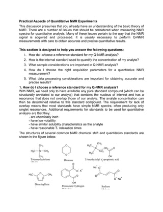
The structures of several common NMR chemical shift and quantitation standards are
shown in the figure below.
CH3 CH3
CH3
Si
CH3
Tetramethylsilane
(TMS)
CD2
CH3
CD2
CH3
Si
CH3
O
OH
Trimethylsilyl d4
-propionic acid
(TMSP)
O
O
Dioxane
Potassium Hydrogen
Phthalate
O
O
-
O
OH
K
+
O
O
-O
O
-
Na
+
Na
+
Sodium
Maleate
Dimethylfura
n
O
CH3CH3

2. TMS and dioxane are chemical shift reference compounds commonly used in organic
solvents. However they do not make good quantitation standards because they suffer
from high volatility. Therefore it is difficult to prepare a standard solution for which the
concentration is known with high accuracy. TMSP is a water soluble chemical shift
reference. While it has improved performance as a quantitation standard compared with
TMS or dioxane, it has been shown to absorb to glass so stock solutions may have
stability problems.1
In addition to the criteria listed above, it is helpful for quantitation
purposes if the compound selected as the standard also has the properties of a primary
analytical standard, for example potassium hydrogen phthalate (KHP), which is
available in pure form, is a crystalline solid at room temperature and can be dried to
remove waters of hydration.
2. How is the internal standard used to quantify the concentration of my analyte?
If an NMR spectrum is measured with care, the integrated intensity of a resonance due
to the analyte nuclei is directly proportional to its molar concentration and to the number
of nuclei that give rise to that resonance.
Integral Area ∝ Concentration Eq. 1
Number of Nuclei
For example the 1
H NMR resonance of a methyl group would have 3 times the intensity
of a peak resulting from a single proton. In the spectrum below for isopropanol, the 2
methyl groups give rise to a resonance at 1.45 ppm that is 6 times greater than the
integrated intensity of the CH resonance at 3.99 ppm. Since this spectrum was
measured in D2O solution, only the resonances of the carbon-bound protons were
detected. The OH proton of isopropanol is in fast exchange with the residual water
(HOD) resonance at 4.78 ppm, therefore a separate resonance is not observed for this
proton.
In this example we compared the relative integrals of the proton resonances of
isopropanol. This information can be very useful for structure elucidation. If we instead
compare the integral of an analyte resonance to that of a standard compound of known
concentration, we can determine the analyte concentration.
Analyte Concentration = Normalized Area Analyte x Standard Concentration Eq. 2
Normalized Area Standard
The direct proportionality of the analytical response and molar concentration is a major
advantage of NMR over other spectroscopic measurements for quantitative analysis.
For example with UV-visible spectroscopy measurements based the Beer-Lambert Law,
absorbance can be related to concentration only if a response factor can be determined
for the analyte. The response factor, called the molar absorptivity in UV-visible
spectroscopy, is different for each molecule therefore, we must be able to look up the
absorptivity or have access to a pure standard of each compound of interest so that a
calibration curve can be prepared. With NMR we have a wide choice of standard
compounds and a single standard can be used to quantify many components of the

3. same solution.
Question 1. A quantitative NMR experiment is performed to quantify the amount of
isopropyl alcohol in a D2O solution. Sodium maleate (0.01021 M) is used as an internal
standard. The integral obtained for the maleate resonance is 46.978. The isopropanol
doublet at 1.45 ppm produces an integral of 104.43. What would you predict for the
integral of the isopropanol CH resonance as 3.99 ppm. What is the concentration of
isopropanol in this solution?
2. What sample considerations are important?
What nucleus should I detect? Just as you might make a choice between measuring
a UV or an IR spectrum, in NMR we often have a choice in the nucleus we can use for
the measurement. A wide range of nuclei can be measured, with the spin ½ nuclei 1
H,
31
P, 13
C, 15
N, 19
F, 29
Si, and 31
P among the most common. However, most quantitative
NMR experiments make use of 1
H, because of the inherent sensitivity of this nucleus
and its high relative abundance (nearly 100%). In addition, as we will see in the next
section, the relaxation properties of nuclei are also important to consider in quantitative
NMR experiments, and compared with many other nuclei like 13
C, 1
H nuclei have more
favorable T1 relaxation times. The choice of the observe nucleus can depend on
whether one seeks universal detection (for organic compounds 1
H and 13
C fall into this
category) or selective detection. For example fluoride ions can be easily detected in
fluorinated water at the sub-ppm level, in large part because of the selectivity of the

4. measurement – one expects to find very few other sources of fluorine in water. Similarly
phosphorous containing compounds like ATP, ADP, and inorganic phosphate can be
detected and even quantified in live cells, tissue or organisms.
How concentrated is my sample? In the Beer-Lambert law you are probably familiar
with from UV-visible spectroscopy, absorbance is directly related to the concentration of
the analyte. Similarly, in NMR the signal we detect scales linearly with concentration.
Since NMR is not a very sensitive method, you would ideally like to work with
reasonably concentrated samples, for protons this means analyte concentrations
typically in the millimolar to molar range, depending on the instrument you will be using.
Other nuclei are less sensitive than protons. The sensitivity issue has two components,
the inherent sensitivity, which depends on the magnetogyric ratio (γ), and the relative
abundance of the nucleus (for example 19
F is 100% abundant, but 13
C is only 1.1% of all
carbon atoms)
What other practical issues do I need to consider? The sensitivity of an NMR
experiment can also be affected by the homogeneity of the magnetic field that the
sample feels. It is normal to adjust the field homogeneity through a process known as
shimming. NMR samples should be free of particulate matter, because particles can
make it difficult to achieve good line shape by shimming. You will also have better luck
with shimming if you have a sample volume sufficient to meet or exceed the minimum
volume recommended by your instrument manufacturer.
3. How do I choose the right acquisition parameters for a quantitative NMR
measurement?
This may not be a big consideration in measuring a UV-visible or IR spectrum; you
generally just walk up to the instrument, place your sample in a sample holder and
make a measurement. However, with NMR there are several parameters, summarized
below, that can have a huge impact on the quality of your results and whether or not
your results can be interpreted quantitatively.
Number of scans. An important consideration is the number of FIDs that are coadded.
Especially for quantitative measurements it is important to generate spectra that have a
high signal-to-noise ratio to improve the precision of the determination. Because the
primary noise source in NMR is thermal noise in the detection circuits, the signal-to-
noise ratio (S/N) scales as the square root of the number of scans coadded. To be 99%
certain that the measured integral falls within + 1% of the true value, a signal-to-noise
ratio of 250 is required. Acquisition of high quality spectra for dilute solutions can be
very time consuming. However, even when solutions have a sufficiently high
concentration that signal averaging is not necessary to improve the S/N, a minimum
number of FIDs (typically 8) are coadded to reduce spectral artifacts arising from pulse
imperfections or receiver mismatch.
Question 2: A solution prepared for quantitative analysis using NMR was acquired by
coaddition of 8 FIDs produces a spectrum with an S/N of 62.5 for the analyte signals.
How many FIDs would have to be coadded to produce a spectrum with an S/N of 250?

5. Acquisition time. The acquisition time (AT) is the time after the pulse for which the
signal is detected. Because the FID is a decaying signal, there is not much point in
acquiring the FID for longer than 3 x T2 because at that point 95% of the signal will have
decayed away into noise. Typical acquisition times in 1
H NMR experiments are 1 – 5
sec.
An interesting feature in choosing an acquisition time is the relationship between the
number of data points collected and the spectral width, or the range of frequencies
detected. Although the initial FID detected in the coil is an analog signal, it needs to be
digitized for computer storage and Fourier transformation. According to Nyquist theory,
the minimum sampling frequency is at least twice the highest frequency detected. The
dwell time (DW) or time between data point sampling is a parameter that is not typically
set by the user, but determined by the spectral width (SW) and the number of data
points (NP).
SW
DW
2
1
= Eq. 4
NPDWAT ×= Eq. 5
Another feature of the acquisition parameters that is important for quantitative
measurements is the digital resolution (DR).
)(realNP
SW
DR = Eq. 6
Almost all spectrometers are designed with quadrature phase detection, which in effect
splits the data points into real and imaginary datasets that serve as inputs for a complex
Fourier transform. It is important to have sufficient digital resolution to accurately define
the peak. Since a typical 1
H NMR resonance has a width at half height (w1/2) of 0.5 to
1.0 Hz, 8-10 data points are required to accurately define the peak. The total number of
data points used in the Fourier transformation and contributing to the digital resolution
can be increased by zero-filling, as described in the section on data processing.
Question 3: A 1
H NMR spectrum was measured using a 400 MHz instrument by
acquisition of 16,384 total data points (8192 real points) and a spectral width of 12 ppm.
What was the acquisition time? Calculate the digital resolution of the resulting
spectrum? Is this digital resolution sufficient to accurately define a peak with a width at
half height of 0.5 Hz?
Receiver gain. The receiver includes the coil and amplifier circuitry that detects and
amplifies the signal prior to digitization by the analog-to-digital converter (ADC). It is
important to set the receiver gain properly so that the ADC is mostly filled, without
overflowing. ADC’s used in NMR typically have limited dynamic range of 16 -18 bits. If
the receiver gain is set too low, only a few bits of the ADC are filled and digitization error
can contribute to poor S/N. If the receiver gain is set too high, (called clipping the FID)
the initial portions of the FID will overflow the ADC and will not be properly digitized. In
this case, resonance intensity can no longer be interpreted in a quantitative manner. In

6. Relaxation
Delay
Variable
Delay
0.16 s
Time (s)
0.16 s
Time (s)
ppm (f1)
34.05.0
ppm (f1)
3.4.05.0
ppm (f1)
34.05.0
ppm (f1)
3.4.05.0
ppm (f1)
3.4.05.0
Fourier Transform
Acquisition180o 90o
Relaxation
Delay
Variable
Delay
0.16 s
Time (s)
0.16 s
Time (s)
ppm (f1)
34.05.0
ppm (f1)
3.4.05.0
ppm (f1)
34.05.0
ppm (f1)
3.4.05.0
ppm (f1)
3.4.05.0
Fourier Transform
0.16 s
Time (s)
0.16 s
Time (s)
ppm (f1)
34.05.0
ppm (f1)
3.4.05.0
ppm (f1)
34.05.0
ppm (f1)
3.4.05.0
ppm (f1)
3.4.05.0
Fourier Transform
Acquisition180o 90o
addition, a lot of spurious signals will appear in the spectrum. For most experiments the
autogain routine supplied by the NMR manufacturer will work well for the initial setup of
the experiment.
Repetition time. The repetition time is the total time between the start of acquisition of
the first FID and the start of acquisition of the second FID. The repetition time is the sum
of the acquisition time and any additional relaxation delay inserted prior to the rf pulse.
Recall that there are two relaxation times in NMR, T1 and T2 (with T1 ≥ T2). If a pulse
width of 90o
is used to signal average multiple FIDs to improve S/N or reduce artifacts,
we generally need to wait 5 x T1 between each acquisition so that the magnetization can
relax essentially completely (by at least 99%) to its equilibrium state. If the repetition
time is less than 5T1, the resonances in the spectrum cannot be simply interpreted in a
quantitative manner and resonance intensity is scaled according to T1.
The inversion-recovery pulse sequence can be used to measure T1 relaxation times. In
this pulse sequence, diagrammed below, the magnetization is inverted by a 180o
pulse.
The relaxation delay at the start of the experiment is selected to assure complete
relaxation between acquisitions.
.
During the variable delay, magnetization relaxes by spin-lattice (T1) relaxation and is
tipped into the transverse plane by the 90o
read pulse. The intensity of the resonances
is measured and then fit to an exponential function to determine the T1 relaxation time.
The figure below shows selected spectra measured for the KHP protons using the
inversion-recovery experiment and the fit of the integral of one of the resonances to
determine the T1 relaxation time of the corresponding proton.
Pulse width. As described in the Basic Theory section, the NMR signal is detected as a
result of a radio frequency (rf) pulse that excites the nuclei in the sample. The pulse
width is a calibrated parameter for each instrument and sample that is typically
expressed in µs. The pulse width can also be thought of in terms of the tip angle, θ, of
the pulse
θ = γB1τ Eq. 7

7. where γ is the gyromagnetic ratio, B1 is the strength of the magnetic field produced by
the pulse and τ is the length of the pulse. For quantitative NMR spectra, 90o
pulses with
a repetition time ≥ 5T1 are typically used since this pulse produces the greatest S/N in a
single scan, although other pulse widths can also be used. For spectra where
qualitative, rather than quantitative analysis is desired, significant time savings can be
obtained by using shorter pulses (i.e. 30o
) since the magnetization takes less time to
recover to its equilibrium state after the pulse. For a more detailed analysis of the
effects of tip angle in quantitative NMR experiments click here
4. What data processing considerations are important for obtaining accurate and
precise results?
Data processing describes operations that are performed to improve spectral quality
after the data has been acquired and saved to disk.
Zero-filling. Zero-filling is the addition of zeros to the end of the FID to increase the
spectral resolution. Because zeros are added, not additional real data points carrying
with them an overlay of noise, zero-filling can improve digital resolution without
decreasing S/N. Another option is to use linear prediction to add data points calculated
from the beginning of the FID where S/N is at its highest.
Apodization. Apodization is the multiplication of the FID by a mathematical function.
Apodization can serve several purposes. Spectral resolution can be improved by
emphasizing the data points at the end of the FID. S/N can be improved by multiplying
the FID by a function that emphasizes the beginning of the FID relative to the later data
points where S/N is poorer. For quantitative NMR experiments, the most common
apodization function is an exponential decay that matches the decay of the FID (a
matched filter) and forces the data to zero intensity at the end of the FID. This function
is often referred to a line broadening, since it broadens the signals based on the time-
ppm (f1)
7.607.707.807.90
-200
-150
-100
-50
0
ppm (f1)
7.607.707.807.90
-100
-50
0
50
ppm (f1)
7.607.707.807.90
-100
-50
0
ppm (f1)
7.607.707.807.90
0
50
100
ppm (f1)
7.5507.6007.6507.7007.7507.8007.8507.9007.950
-50
0
50
ppm (f1)
7.407.507.607.707.807.90
0
50
100
150
0 s
2 s
2.5 s
3.5 s
4 s
20 s
Representative Inversion-recovery Spectra for KHP
ppm (f1)
7.607.707.807.90
-200
-150
-100
-50
0
ppm (f1)
7.607.707.807.90
-100
-50
0
50
ppm (f1)
7.607.707.807.90
-100
-50
0
ppm (f1)
7.607.707.807.90
0
50
100
ppm (f1)
7.5507.6007.6507.7007.7507.8007.8507.9007.950
-50
0
50
ppm (f1)
7.407.507.607.707.807.90
0
50
100
150
0 s
2 s
2.5 s
3.5 s
4 s
20 s
Representative Inversion-recovery Spectra for KHP
0 5 10 15 20
-40
-30
-20
-10
0
10
20
30
40
Intensity
Inversion Recovery Delay (s)
Fit of Inversion Recovery Data to Determine T1
1
20
T
t
eII
−
−=

8. constant of the exponential decay. This trade-off between S/N and spectral resolution is
not restricted to NMR and is common to many instrumental methods of analysis.
Integration regions. Because NMR signals are Lorentzians, the resonances have long
tails that can carry with them significant amounts of resonance intensity. This is
especially problematic when the sample is complex containing many closely spaced or
overlapped signals, or when the homogeneity of the magnetic field around the sample
has not been properly corrected by shimming. For a Lorentzian peak with a width at
half-height of 0.5 Hz, integration regions set at 3.2 Hz or 16 Hz on either side of the
resonance would include approximately 95% or 99% of the peak area, respectively.
Note that this analysis does not include the 13
C satellites which account for an additional
1.1% of the intensity of carbon-bound protons in samples containing 13
C at natural
abundance. In cases where resonances are highly overlapped, more accurate
quantitative analysis can often be achieved by peak fitting rather than by integration.
An alternative approach utilizes 13
C decoupling during the acquisition of the proton
spectrum to collapse the 13
C satellites so that this signal is coincident with the primary
1
H-12
C resonance.2, 3
This relatively simple approach requires only that the user has
access to a probe (for example a broadband inverse or triple resonance probe) that
permits 13
C decoupling.
Baseline correction. NMR integrals are calculated by summation of the intensities of
the data points within the defined integration region. Therefore, a flat spectral baseline
with near zero intensity is required. This can be achieved in several ways; the most
common is selecting regions across the spectrum where no signals appear, defining
these as baseline and fitting them to a polynomial function that is then subtracted from
the spectrum.
References
1. D.A. Jayawickrama, C.K. Larive, Anal. Chem. 71:2117-2112 (1999).
2. The Quantitative NMR Portal, http://tigger.uic.edu/~gfp/qnmr/
3. G. F. Pauli, B. U. Jaki, D. C. Lankin “A Routine Experimental Protocol for qHNMR
Illustrated with Taxol“ J. Nat. Prod. 70:589-595 (2007).