SlideShare a Scribd company logo
1 of 78
Chad Jones uses two different methods in predicting how the
World Income Distribution (WID) will evolve in the future. The
first approach he uses is based on the findings of the Solow
model, which Jones then uses to say that it is up to the
fundamentals of a country such as its savings rate and
population growth rate, that determines how fast it will grow in
the future. He plugs in the fundamentals he finds of a country
from 1988 to project the future levels of income distribution,
and determine whether or not there has been change and in what
direction (increase or decrease). The criticism of this approach,
however, is that it assumes that the fundamentals of savings rate
and population growth rate, for example, are fixed at 1988
levels.
The second approach Jones takes is not reliant on the Solow
model, and is rather called the Markov Transitional Matrix.
Essentially, Jones here classifies the data he has, either within a
country's household income distribution as we learned in class
or across different countries, as bottom tier, middle tier, or top
tier. Then, depending on how much of the data falls outside of
the central diagonal formed by the data, Jones determines
whether the country or countries experiences an
increase/decrease/stagnation in income distribution levels in the
future. The criticism about this approach, however, is that it
assumes that the distributions of growth rates across countries
would stay constant in the future as they were in the period
between 1960 and 1988, which is a very big detail to assume
and would skew the findings coming out of this approach.
Lant Pritchett also tries to explain the idea of convergence
through two separate methods. Because the only evidence that
existed at the time was based on OECD countries or more
rich/developed countries, Pritchett attempts to influence the
literature by accounting for the poorer countries. He does this
by finding what the lowest level of GDP/capita is in our modern
day by looking at the poorest of countries in our time. He then
assigns this level to countries that data could not be found for in
the past, because Pritchett states that countries could not exist if
they did not even meet this threshold for GDP/capita. This
number is $250. The second method he uses is to prove that
assigning this $250 for poor countries in the past is not
outrageous. He does this by determining the relationship
between caloric consumption and GDP/capita and then finding
what the basic number of calories needed to survive was, which
was around 2,400 calories. Pritchett then plugged 2,400 into his
relationship between caloric consumption and GDP/capita to
back out what the level of GDP/capita would be in countries
who only managed to meet 2,400 calories/day, which was the
minimum subsistence level. The number he got for GDP/capita
using this method was between $250-$280, which confirms his
ability to plug this in for poor countries that did not have data
in the past. A criticism of this approach is that there will never
a feasible way to determine convergence, because regardless of
the minimum GDP/capita you place for the poor countries,
empirically the model will show that the poor countries can
never and will never catch up to the richer countries. We saw
this in the last example in class, when countries were placed at
$100, they still weren't reaching the 2% growth rate that rich
countries were reaching yearly, symbolizing that these poorer
countries could not catch up regardless of their low GDP/capita
levels.
Journal of Economic Perspectives—Volume 11, Number 3—
Summer 1997—Pages 19–36
On the Evolution of the World Income
Distribution
Charles I. Jones
H
ow rich are the richest countries in the world relative to the
poorest? Are
poor countries catching up to the rich countries or falling
further be-
hind? How might the world income distribution look in the
future?
These questions have been the subject of much empirical and
theoretical work over
the last decade, beginning with Abramovitz (1986) and Baumol
(1986), continuing
with Barro (1991) and Mankiw, Romer and Weil (1992), and
including most re-
cently work by Quah (1993a, 1996). This paper provides one
perspective on this
literature by placing it explicitly in the context of what it has to
say about the shape
of the world income distribution. We begin in the first section
by documenting
several empirical facts concerning the distribution of GDP per
worker across the
countries of the world and how this distribution has changed
since 1960.1
The main part of the paper attempts to characterize the future of
the world
income distribution using three different techniques. First, we
use a standard
growth model to project the current dynamics of the income
distribution forward,
assuming the policies in place in each country during the 1980s
continue. One can
interpret this exercise as forecasting the near-term income
distribution. The results
indicate that the near-term income distribution looks broadly
like the current dis-
tribution. However, there are some notable exceptions,
primarily at the top of the
income distribution, where a number of countries are predicted
to continue to
converge toward and even overtake the United States as the
richest country in the
world.
Second, we exploit insights from the large literature on cross-
country growth
1For a related review of the facts, see Parente and Prescott
(1993) and Jones (forthcoming).
• Charles I. Jones is Assistant Professor of Economics, Stanford
University, Stanford, Cali-
fornia. His e-mail address is [email protected]
20 Journal of Economic Perspectives
regressions following Barro (1991) and Mankiw, Romer and
Weil (1992). An im-
portant finding of this literature is that one can interpret the
variation in growth
rates around the world as reflecting how far countries are from
their "steady state"
positions. Korea and Japan have grown rapidly because their
steady state positions
in the income distribution are much higher than their current
positions. Venezuela
has grown slowly because the reverse is true. We use this
insight to provide a second
way of predicting where countries are headed based on current
policies.
Finally, we step back and consider how the steady states toward
which countries
are headed are themselves changing. The evidence from the last
30 years suggests
that growth miracles are occurring more frequently than growth
disasters and that
the relative frequency of miracles has increased. Projecting
these dynamics forward
indicates that the long-run world income distribution involves a
substantial im-
provement in the incomes of many countries. For example in
1960, 60 percent of
countries had incomes less than 20 percent of incomes in the
richest country. In
the long run, the empirical results indicate that the fraction of
"poor" countries
will fall from 60 percent to only 27 percent.
Facts
Before examining several facts about the world income
distribution, it is worth
pausing for a moment to consider which definition of income to
use. GDP per
capita seems like a natural definition if one is interested in an
important determi-
nant of average welfare. However, in many developing
countries, nonmarket pro-
duction is quite important, leading GDP per capita to understate
true income in
these countries. A coarse correction for this problem is to focus
on GDP per worker.
Both the numerator and the denominator then correspond to the
market sector.
To the extent that wages are equalized at the margin between
the market and
nonmarket sectors, this is a natural measure of income, and it is
the one employed
in most of this paper.
The world distribution of GDP per worker has changed
substantially during
the post-World War II period. Figure 1 plots the density of GDP
per worker relative
to the United States in 1960 and 1988 for 121 countries.2
Roughly speaking, the
more countries there are at a particular level of income, the
higher the density will
be at that point in the figure. The 121-country sample, which
includes all countries
for which Summers and Heston (1991) report real GDP per
worker in both years,
will make up the "world" for the purposes of this paper. The
most notable
omissions are several Eastern European economies and several
economies in the
Middle East for which data are not reported in 1960.
A number of features in this figure deserve comment. First, the
distribution is
2 T h e data are from the Penn World Tables Mark 5.6 update of
Summers and Heston (1991) and
therefore are in principle corrected for differences in purchasing
power across economies. The density
estimates are computed using a Gaussian kernel with a
bandwidth chosen as .9AN–1/5 where A is the
standard deviation of the data and N is the number of
observations.
Charles I. Jones 21
Figure 1
World Income Distribution, 1960 and 1988
wide. In 1988, for example, the ratio of the income in the
richest country (the
United States) to the poorest country (Myanmar) was 35.
Second, the 1960 distri-
bution is single-peaked and looks roughly normal, although the
tails are too thick.
In contrast, the distribution in 1988 exhibits "twin-peaks," to
use the appellation
coined by Quah (1993a). This change reflects a shift in the mass
of the distribution
away from the middle and toward the ends. In particular, the
"hump" in the 1960
distribution between about 5 and 30 percent of U.S. income has
shifted upward
into the 20 to 65 percent range. Finally, the world income
distribution is wider in
1988 than it was in 1960, both at the top and at the bottom.
What cannot be seen in the figure is the general growth in GDP
per worker
throughout the world. Though this paper is almost entirely
about relative incomes,
it is important to remember that in absolute terms, income
growth is a prevalent
feature around the world. For example, U.S. GDP per worker
grew at an average
annual rate of 1.4 percent from 1960 to 1988. In other words, if
in Figure 1 we
plotted actual instead of relative incomes, the 1988 distribution
would be shifted
noticeably to the right. Nevertheless, not all countries
experienced positive growth.
GDP per worker actually declined from 1960 to 1988 in 11
percent of the countries.
Throughout this paper, we will consider incomes relative to
U.S. income; that
is, we will focus on the GDP per worker of the countries of the
world divided by
U.S. GDP per worker. The choice of the denominator is an
important one, and
U.S. income is chosen for several reasons. First, the United
States had the highest
GDP per worker in both 1960 and 1988, so the units of relative
income are readily
interpreted. Second, U.S. growth has been relatively steady over
this 30-year period.
Finally, it is natural to think of the U.S. economy as lying close
to the technological
frontier. Therefore, U.S. growth is probably a reasonable proxy
for the growth rate
of the technological frontier. These considerations indicate that
the U.S. economy
22 Journal of Economic Perspectives
is "well-behaved" and that normalizing by U.S. income will not
distort our view of
the income distribution.
One drawback of Figure 1 is that individual countries cannot be
identified.
Figure 2 helps to address this concern by plotting GDP per
worker relative to the
United States in 1960 and in 1988 on a natural log scale.3
Changes in the world
distribution of income are then illustrated by departures from
the 45-degree line.
Countries with GDP per worker greater than about 15 percent of
U.S. income in
1960 typically experienced increases in relative income. These
countries corre-
spond to the shift in the mass of the income distribution toward
the top in Figure
1. On the other hand, many countries with relative incomes of
less than 10 or
15 percent in 1960 experienced a decrease in relative income
over this period. They
grew more slowly than did the United States and more slowly
than did most of the
countries above the 15 percent mark. These are the countries
that make u p the
peak at the lower end of the income distribution. One way of
interpreting these
general movements is that there has been some convergence or
"catch-up" at the
top of the income distribution and some divergence at the
bottom.
Figure 2 also allows us to identify the growth miracles and
growth disasters of
this 28-year period. Hong Kong (HKG), Singapore (SGP), Japan
(JPN), Korea
(KOR) and Taiwan (OAN) all stand out as growth miracles,
having increased their
relative incomes substantially. For example, Hong Kong,
Singapore and Japan grew
from about 20 percent of U.S. GDP per worker in 1960 to
around 60 percent in
1988. Korea rose from 11 percent to 38 percent. Several less
well known growth
miracles are also noteworthy. Relative income in Botswana
(BWA) increased from
5 percent to 20 percent, in Romania (ROM) from 3 percent to 12
percent, and in
Lesotho (LSO) from 2 percent to 6 percent.
A large number of the growth disasters—countries that
experienced large de-
clines in relative incomes—are located in sub-Saharan Africa.
Chad (TCD), for
example, fell from a relative income of 8 percent to 3 percent.
However, growth
disasters outside Africa are also impressive. For example,
Venezuela (VEN) was the
third richest economy in the world in 1960 with an income
equal to 84 percent of
U.S. income. By 1988, relative income had fallen to only 55
percent.
The facts about the world income distribution so far have
concerned the be-
havior of incomes in terms of countries. While this is a common
way to view the
data, it can be misleading: for example, if we drew national
borders differently—
for example, so that each of the 50 U.S. states were a separate
country—the shape
of the densities in Figure 1 would look different. An alternative
approach is to
weight each country by its population. The unit of observation
is then a person
instead of a country.4 The most important fact to note in this
regard is that roughly
40 percent of the world's population lives in China (23 percent
in 1988) and India
(17 percent in 1988). The experience of these two countries
largely determines
3 A complete guide to the country codes used in this figure can
be found on the World Wide Web at
http://www.stanford.edu/~chadj/growth.html.
4 O f course, this exercise says nothing about changes in the
income distribution within a particular
country.
On the Evolution of the World Income Distribution 23
Figure 2
Relative Y/L, 1960 vs. 1988
(log scale)
what happens to the "typical" poor person in the world. In
contrast, less than
10 percent of the world's population lives in the 39 countries
that make up sub-
Saharan Africa.
Figure 3 plots the density of GDP per worker relative to the
United States,
weighted by population. In comparing this figure to Figure 1,
one sees the over-
whelming importance of India and China. While the distribution
of countries has
exhibited some divergence at the bottom, the same is not true
for the distribution
weighted by population. Both China and India have grown faster
than the United
States in the last three decades, leading to some catch-up at the
bottom of the
income distribution weighted by population. The catch-up in the
top part of the
income distribution also remains evident in Figure 3.
The cumulative distribution of GDP per worker by population—
that is, the
area under the density—provides additional information that is
helpful in inter-
preting Figure 3. In terms of the cumulative distribution, 50
percent of the world's
population lives in countries in which GDP per worker is about
10 percent of that
in the United States. To be more exact, the income of the
country containing the
median person has improved from 8.1 percent of U.S. income in
1960 to
11.8 percent in 1988. Improvements for people higher up in the
distribution have
24 Journal of Economic Perspectives
Figure 3
Density of GDP Per Worker Weighted by Population
been even more substantial. The 75th percentile of the
population lived in a country
with 22.5 percent of U.S. income in 1960, but 40.3 percent in
1988. The 90th
percentile of the population lived in a country with 59.2 percent
of U.S. income in
1960, and 79 percent in 1988.
The Assumption of Similar Long-Term Growth Rates
The remainder of this paper considers various techniques for
making state-
ments about the future shape of the world income distribution.
First, however, there
is an important issue to consider. The world income distribution
will only settle
down to a stable, nondegenerate distribution if all countries
eventually grow at the
same rate. Why? Well, suppose one thinks growth in Japan will
permanently be
higher than growth in the United States. In that case, the ratio
of Japanese to U.S.
income will diverge to infinity. If this is the way the world
works, one might be more
interested in the long-run distribution of growth rates than in
incomes. However,
I will argue here that in the long run, all countries are likely to
share the same rate
of growth.
This assertion may seem counterintuitive. After all, growth
rates of output
per worker over long periods of time do differ substantially, and
there may be
an initial inclination to believe that the endogenous growth
literature has pro-
vided ample evidence against this hypothesis. Nevertheless,
there are both con-
ceptual and empirical reasons to think that most countries are
likely to share
the same rate of growth in the long run. The conceptual reason
is most persua-
Charles I. Jones 25
sive and has been presented in several recent papers (Eaton and
Kortum, 1994;
Parente and Prescott, 1994; Barro and Sala-i-Martin, 1995;
Bernard and Jones,
1996). Following the recent endogenous growth literature, let us
assume that
the engine of growth is technological progress: output per
worker grows in the
long run because of the creation of ideas. Ideas diffuse across
countries, perhaps
not instantaneously, but eventually. Belgium does not grow only
or even largely
because of the ideas created by Belgians, but rather a
substantial amount of
growth in Belgian output per worker is due to ideas invented
elsewhere in the
world. In this framework, the fact that countries of the world
eventually share
ideas means that their incomes cannot get infinitely far apart.
All countries even-
tually grow at the average rate of growth of world knowledge,
as shown in each
of the papers cited above.
Which brings us to the empirical reason. What do we make of
the large em-
pirical variation in growth rates? Japan, for example, grew at an
average rate of
5.1 percent per year between 1960 and 1988 while the United
States grew only at
1.4 percent. Or consider an even longer horizon using the GDP
per capita data
reported by Maddison (1995). Over the century and a quarter
spanning 1870 to
1994, the United States grew at an average rate of 1.8 percent
per year while the
United Kingdom grew only at 1.3 percent.
In fact, such differences—even over 125 years—are not
inconsistent with the
hypothesis that all countries share a common long-run growth
rate. The resolution
of this apparent inconsistency is transition dynamics. To the
extent that countries
are changing position within the world income distribution,
their average growth
rate can be faster or slower than the growth rate of world
knowledge over any finite
period. This point is illustrated clearly by a closer look at the
U.S. and U.K. evidence
for the last century.
Figure 4 plots the log of GDP per capita in the United States
and United
Kingdom from 1870 to 1994 using the data from Maddison
(1995). As men-
tioned above, average growth in the United States has been a
half a percen-
tage point higher than in the United Kingdom over this 125-year
period. How-
ever, as the figure shows, nearly all of this difference is
accounted for by the
pre-1950 experience. Between 1870 and 1950, the U.S. economy
grew at
1.7 percent while growth in the United Kingdom was a
comparatively
sluggish 0.9 percent. This growth performance occurred as the
United States
overtook the United Kingdom as the world's richest country
around the turn
of the century. Since 1950, however, average growth rates have
been almost
identical, with the United States growing at 1.95 percent and the
United
Kingdom growing at 1.98 percent. Forecasters who in 1950
expected the large
growth differentials of the preceding 70 years to continue were
clearly
mistaken.
Similarly, the fact that Japan has grown faster than the United
States since 1950
says very little about whether or not these two economies will
grow at the same rate
in the long run. Rather, in a world where Japan and the United
States have a
common long-run growth rate, the experience of the last half-
century is evidence
that Japan is moving " u p " in the income distribution.
26 Journal of Economic Perspectives
Figure 4
Income in the United States and United Kingdom
(log scale)
The Future of the Global Income Distribution
Under the assumption that all countries grow at the same
average rate in the
long run, there are a number of ways to make statements about
the eventual shape
of the income distribution. The remainder of this paper employs
three such tech-
niques. First, we examine the predictions generated from a
standard, well-known
growth model due to Solow (1956). Second, we use a prediction
based on transition
dynamics. And finally, we employ a statistical technique that
looks at the frequency
of growth miracles and growth disasters.
Projecting from Current Investment Levels
The Solow (1956) growth model predicts that the level of output
per worker
in an economy in the long run is a function of the rate of
investment in capital,
the growth rate of the labor force, and the level of technology.
5
Statements about
the future of the income distribution can be made if we can
make statements about
the future of investment rates, population growth rates, and
(relative) technology
levels. Notice that nothing really hinges on our following Solow
in assuming ex-
ogenously given and constant investment rates and population
growth rates. Pro-
vided these variables "settle down" in steady state to some
constant value (which
is nearly a definition of the steady state), what we really need
empirically is to be
5
Mathematically, y(t) = (s/(n + g + δ ) )
α / 1 - α
A ( t ) , where s is the investment rate, n is the population
growth rate, δ is the constant rate at which capital depreciates,
α is capital's share in production, and
A(t) is the level of labor-augmenting technology, which is
assumed to grow at the constant, exogenous
rate g.
On the Evolution of the World Income Distribution 27
able to predict where these variables are going to settle. The
Solow model then tells
us how to map these values into steady state incomes.
Jones (1997) follows this line of reasoning in a more general
model that in-
corporates human capital as well as physical capital. A simple
way of predicting
where investment rates and population growth rates will settle is
to assume that the
rates that prevailed in the 1980s will persist. Of course, this
simple method ignores
the fact that investment rates, for example, may be affected by
the transition dy-
namics of the economy. Moreover, what this exercise cannot
predict are underlying
changes in policy, which are presumably very important in the
actual evolution of
the income distribution. Still, this is a useful benchmark to
consider. Later sections
will address these other concerns.
Figure 5 plots steady state relative incomes based on this
forecasting exercise
against relative incomes in 1988 for 74 countries.6 Two features
of Figure 5 stand
out. First, broadly speaking, the 1988 distribution is quite
similar to the distribution
of steady states. Uganda (UGA) and Malawi (MWI) are not poor
because of tran-
sition dynamics. Rather, they are poor because investment rates
are low and tech-
nology levels are low. (Population growth rates are also high,
but a little analysis
illustrates that changes in population growth rates have
relatively small effects in
most neoclassical models.) Based on recent experience in the
1980s, there is no
reason to expect these broad features driving the world income
distribution to
change in the near future.
Second, this similarity is less pronounced at the top of the
income distribution,
where countries continue to "catch up" to the United States,
than it is at the
bottom. One notable exception is India (IND), which is
predicted to grow from a
relative income of 9 percent in 1988 to 13 percent based on
policies in place in the
1980s. Similarly, Malaysia (MYS), Korea, Hong Kong and
Singapore are all pre-
dicted to continue to grow faster than the United States during a
transition to
higher relative incomes, as are a number of OECD economies
like Spain (ESP),
Italy (ITA) and France (FRA). In fact, according to this
particular exercise, a
number of countries such as Singapore, Spain, France and Italy
are predicted to
surpass the United States in GDP per worker. While the exact
location of particular
countries is somewhat sensitive to assumptions, this general
feature that the United
States is not expected to retain its lead in output per worker is
robust. The expla-
nation is simple. Ignoring differences in technology for the
moment, differences
in income are driven by differences in investment rates in
physical and human
capital. The United States is one of the leaders in human capital
investment
(though not by much), but its investment rate in physical capital
is substantially
lower than are investment rates in a number of other countries.
A high U.S. tech-
nology level helps, but it is insufficient to compensate for the
lower U.S. investment
6Specifically, the exercise assumes a common capital share of
1/3 across countries. Educational attain-
ment is assumed to augment labor, and a common rate of return
to schooling of 10 percent is used.
Investment rates, schooling enrollment rates and population
growth rates from the 1980s and the level
of (labor-augmenting) total factor productivity from 1988 are
used in the computation. See Jones (1997)
for more details.
28 Journal of Economic Perspectives
Figure 5
Steady State Incomes, Based on Current Policies
rate. It is largely these differences that are driving the
differences in incomes at the
top of the distribution.7
Transition Dynamics and Steady State Incomes
A second way of estimating the shape of the steady state income
distribution
exploits recent work in the cross-country growth literature.
According to this work,
one of the most persuasive explanations for why some countries
have grown faster
than others over long periods of time is transition dynamics.
The further a country
is below its steady state position in the income distribution, the
faster the country
should grow. I will refer to this as the principle of transition
dynamics. This principle
can be found in the Solow and Ramsey growth models, as well
as in models that
emphasize the importance of technology transfer and the
diffusion of ideas.8
7 Jones (1997) considers several scenarios to check the
robustness of these findings, including models
in which technology levels converge, a demographic transition
leads to identical population growth rates
around the world, human capital investment rates converge, and
physical capital flows internationally to
equalize returns.
8 O n l y the simplest growth models in which the dynamics are
driven by foregoing consumption to invest
output in physical capital, human capital, or research generally
obey the principle as written (for ex-
Charles I. Jones 29
According to this principle, the growth rate of the economy is
proportional to
the gap between the country's current position in the income
distribution and its
steady state position. In an unfortunate choice of terminology,
the factor of pro-
portionality is sometimes called the "speed of convergence."
This phrase uses the
word convergence in the mathematical sense of a sequence of
numbers converging
to some value. It describes the rate at which a country closes the
gap between its
current and steady state positions in the income distribution.
This use is unfortu-
nate because it seems to suggest that this equation has
something to do with dif-
ferent countries getting closer together in the income
distribution, which is not the
case (at least not directly). With this definition, the principle of
transition dynamics
can be stated as
Growth rate of relative income = Speed of convergence
× Percentage gap to own steady state.
For example, suppose a country has a GDP per worker relative
to the United States
of 0.4 and a steady state value equal to 0.5. This represents a 20
percent gap. If the
speed of convergence is 5 percent per year, then the country can
expect its relative
income to grow at 1 percent per year. Its actual GDP per worker
will then grow at
1 percent plus the underlying growth rate of world technological
progress (assum-
ing the United States has reached its steady state).9
This relation has been exploited by the cross-country growth
literature to ex-
plain differences in growth rates. The numerous right-hand side
variables included
in such regressions, in addition to the initial GDP per worker
variable, are an at-
tempt to measure the gap between initial income and the steady
state position of
the country in the world income distribution. A key parameter
estimated by these
regressions is the speed of convergence. For example, a number
of authors such as
Mankiw, Romer and Weil (1992) and Barro and Sala-i-Martin
(1992) have
documented using econometric techniques the well-known "2
percent" speed of
convergence. Other authors, however, have recently argued for
faster rates of con-
vergence.10 The standard Solow model implies a speed of
convergence of about 6
percent for conventional parameter values. Alternatively, in a
model that incorpo-
rates the diffusion of technology across countries, the speed of
convergence is re-
lated to the rate of diffusion.
In general, the authors in the cross-country growth literature
have not exam-
ined the shape of the steady state world income distribution
implied by their re-
gressions. However, the principle of transition dynamics
suggests a simple, intuitive
way to calculate the distribution of steady states. Instead of
using the principle to
ample, Mankiw, Romer and Weil, 1992). More sophisticated
models require more than one state variable
and cannot typically be reduced to so simple a formulation,
although a similar relation often holds,
either as an approximation or when applied to a slightly
different variable such as total factor productivity.
9Mathematically, the principle of transition dynamics is dlog
(t)/dt = λ(log * – log (t)) where is
relative income, * denotes the steady state value of relative
income, and λ is the "speed of convergence."
1 0
F o r example, see the work employing panel data of Islam
(1995) and Caselli, Esquivel and Lefort
(1996).
30 Journal of Economic Perspectives
estimate speeds of convergence in a regression, we can simply
impose alternative
values. Then, data on growth rates from 1960 to 1988 and initial
incomes in 1960
can be used to back out the implied steady states.11 To the
extent that countries
roughly obeyed a stable principle of transition dynamics over
this 28-year period,
we can calculate the targets toward which they were growing.
Figure 6 reports the results of this exercise for several cases,
corresponding to
speeds of convergence of 2 percent, 4 percent and 6 percent. In
general, the steady
state distributions are determined as follows. Countries that
have grown faster than
the United States has over the 28-year period are predicted to
continue to increase
relative to the United States; countries that have grown more
slowly are predicted
to continue to fall. The extent to which the changes continue is
determined by the
speed of convergence. If this speed is slow, as in the first panel
of Figure 6, then
steady states must be far away in order to explain a given
growth differential, im-
plying large additional changes in the income distribution. On
the other hand, if
the speed is fast, say at 6 percent as in the last panel, then smal l
deviations from
the steady state can generate large growth differences; as a
result, the current dis-
tribution looks quite similar to the steady state distribution.
Looking more carefully at the first panel of the figure, the
steady state relative
incomes for a number of countries seem implausibly large with
a 2 percent speed
of convergence. A number of East Asian countries are predicted
to have incomes
of more than 150 percent of U.S. income. The explanation for
this prediction is
that these countries have grown very rapidly for 30 years; with
a very low speed of
convergence, the only way to obtain such rapid growth rates is
if the countries are
extremely far from their steady states. In contrast, the steady
states computed with
a 4 percent or a 6 percent rate of convergence seem more
reasonable.12
The Very Long-Run Income Distribution
So far, we have considered the future of the income distribution
under the
assumption that the policies currently in place in each country
continue, so that
countries are growing toward constant targets. This has a
number of advantages.
For example, it allows us to infer the position within the income
distribution toward
which each country is headed. It also has the flavor of
forecasting the near future.
However, much of the movement of countries within the income
distribution
presumably occurs as a result of policy changes within a
country (broadly inter-
preted to include institutional changes). Japan, for example, had
an income of
roughly 20 percent of that in the United States from 1870 until
World War II. After
the substantial reforms following World War II, we see
enormous increases in Jap-
1 1 To be more precise, we first integrate the equation in
footnote 9 and compute the average growth
rate, as in Mankiw, Romer and Weil (1992). The resulting
equation can be solved for * as a function
of the data.
1 2This result suggests one possible limitation of the exercise.
The calculation assumes that the growth
dynamics for 30 years are driven by a one-time increase in the
gap between current income and steady
state income. Instead, perhaps the steady states for these
economies have shifted upward several times
over the last 30 years. Some calculations reveal that this
alternative does not help as much as one might
suspect.
On the Evolution of the World Income Distribution 31
Figure 6
Steady States Implied by Transition Dynamics
anese relative income far beyond recovery back to the 20
percent level. On the
other side, there is the famous example of Argentina, a
relatively rich country dur-
ing the early part of the twentieth century, but with income in
1988 of only
42 percent of that of the United States. Much of this decline is
attributable to the
32 Journal of Economic Perspectives
Table 1
Frequency of Growth Miracles and Growth Disasters
disastrous policy "reforms" of the Perón era (De Long, 1988,
and the references
there).
Predicting when and where such large changes in institutions
and economic
policies will occur is extremely difficult, if not impossible;
certainly, it requires de-
tailed knowledge of a particular economy. However, predicting
the frequency with
which such changes are likely to occur somewhere in the world
during a decade is
somewhat easier: we observe a large number of countries for
several decades and
can simply count the number of growth miracles and growth
disasters.
One way of making this count is provided in the first row of
Table 1. The 121
countries are classified according to how fast they grew from
1960 to 1988. The
somewhat arbitrary cutoffs for fast and slow growth are defined
as one percentage
point faster and slower than U.S. growth. Because its growth
rate is a reasonable
proxy for the growth rate of the world's technological frontier,
the United States is
a natural benchmark for this exercise. The first row of the table
clearly illustrates
one of the key facts about the world income distribution: rapid
growth has been
significantly more common over the last 30 years than slow
growth. For example,
40 percent of countries experienced fast growth over this
period, while only 15
percent of countries experienced slow growth. This general
result was also apparent
in Figure 2. Looking back at this figure, one sees that there are
more countries
moving up in the distribution than moving down. There are
more Italys than
Venezuelas.
The second part of the table divides countries into six intervals,
based on their
GDP per worker in 1960. For example, the intervals correspond
to countries with
income less than 5 percent of U.S. income, less than 10 percent
but more than 5
percent, and so on. The variable indicates a country's GDP per
worker measured
as a fraction of U.S. income. This part of the table documents
that fast growth and
slow growth occur at roughly the same frequency at the bottom
of the income
distribution; if anything, slow growth is more common. For
countries with incomes
Charles I. Jones 33
Table 2
World Income Distributions, Using Markov Transition Method
of more than 10 percent of U.S. GDP per worker, however, the
frequency of rapid
growth rises markedly. The clear implication is that once
countries make it out of
the lowest income categories, significant upward movements in
the income distri-
bution are much more common than large downward
movements.
Motivated by this data on the frequency of fast and slow
growth, we can provide
a forecast of the very long-run income distribution. Table 2
follows the approach
of Quah (1993a,b) based on Markov transition analysis. As in
Table 1, we sort
countries into intervals based on their 1960 levels of income
relative to the world's
leading economy, the United States during recent decades.13
Then, using annual
data from 1960 to 1988 for the 121-country sample, we
calculate the probabilities
that countries will move from one interval to another. Finally,
using these sample
probabilities, we compute an estimate of the long-run
distribution of incomes.14
The sense in which this computation is different from the
forecasts of the
income distribution in previous sections of the paper is worth
emphasizing. Previ-
ously, we computed the steady state toward which each
economy seems to be
headed and examined the distribution of the steady states based
on current policy
regimes. Here, the exercise recognizes that all countries may be
subject to policy
changes that shift their steady state positions. Therefore, the
computation empha-
sizes a longer-term view of the income distribution. Moreover,
instead of focusing
on any particular country, we focus on the shape of the
distribution as a whole. It
turns out that in the long-run distributions computed using this
approach, there is
a positive probability of any country spending some time in any
interval. This is
because there is some probability that a country, no matter how
rich or poor, will
experience a large policy disaster or policy reform.
13I use the United States as the world's leading economy for the
entire 1960-1988 period despite the
fact that a number of oil-producing economies had higher GDP
per worker in the late 1970s.
14Mathematically, the computation is easily illustrated. First,
we estimate the transition probabilities of
a Markov transition matrix using sample data. Multiplying this
matrix by a vector that corresponds to
the current distribution yields an estimate of the distribution
during the next period. Doing this many
times yields an estimate of the long-run distribution.
34 Journal of Economic Perspectives
Table 2 shows the distribution of countries across the income
intervals in 1960
and 1988 as well as estimates of the future distributions. The
basic changes from
1960 to 1988 have already been documented. There has been
some "convergence"
toward U.S. income at the top of the income distribution, and
this phenomenon is
evident in the table. The long-run distribution, according to the
Markov results,
strongly suggests that this convergence will play a dominant
role in the continuing
evolution of the income distribution. For example, in 1960 only
3 percent of coun-
tries had more than 80 percent of U.S. income, and only 20
percent had more than
40 percent of U.S. income. In the long run, according to the
results, 19 percent of
countries will have relative incomes of more than 80 percent of
the world's leading
economy and 49 percent will have relative incomes of more than
40 percent. Similar
changes are seen at the bottom of the distribution: in 1988, 17
percent of countries
had less than 5 percent of U.S. income; in the long run, only 8
percent of countries
are predicted to be in this category. This latter result is of
interest in light of the
finding reported in Table 1 that large upward and downward
movements occur
with roughly the same frequency at the bottom of the
distribution. The long-run
results here suggest that there is no development trap into which
the poorest coun-
tries will be permanently condemned. The columns in the table
labeled "2010"
and "2050" provide some indication of how long it takes before
this long-run dis-
tribution is reached.
The world income distribution has been evolving for centuries.
Why doesn't
the long-run distribution look roughly like the current
distribution? This is a broad
and important question. The fact that the data say that the long-
run distribution is
different from the current distribution indicates that something
in the world con-
tinues to evolve: the frequency of growth miracles in the last 30
years must have
been higher than in the past, and there must have been fewer
growth disasters.
One possible explanation of this result is that society is
gradually discovering
the kind of institutions and policies that are conducive to
successful economic
performance, and these discoveries are gradually diffusing
around the world. To
take one example, Adam Smith's An Inquiry into the Nature and
Causes of the Wealth
of Nations was not published until 1776. The continued
evolution of the world in-
come distribution could reflect the slow diffusion of capitalism
during the last 200
years. Consistent with this reasoning, the world's experiments
with communism
seem to be coming to an end only in the 1990s. Perhaps it is the
diffusion of wealth-
promoting institutions and infrastructure that accounts for the
continued evolution
of the world income distribution. Moreover, there is no reason
to think that the
institutions in place today are the best possible institutions.
Institutions themselves
are simply ideas, and it is quite likely that better ideas are out
there waiting to be
found. Over the broad course of history, better institutions have
been discovered
and implemented. The continuation of this process at the rates
observed during
the last 30 years would lead to large improvements in the world
income distribution.
Using the Markov methods, we can conduct some other
experiments that
are informative. For example, we can calculate the likelihood of
large move-
ments within the income distribution. Consider first the
frequency of growth
miracles. T h e "Korean e x p e r i e n c e " is not all that
unlikely. A country in the
On the Evolution of the World Income Distribution 35
10 percent bin will move to an income level in the 40 percent
bin or higher with
a 10 percent probability after 37 years. The same is true of the
"Japanese ex-
perience:" a country in the 20 percent bin will move to the
richest category with
a 10 percent probability after 50 years. Given that there are a
large number of
countries in these initial categories, one would expect to see
several growth
miracles at any point in time.
One can also speculate on the frequency of large movements in
the opposite
direction. A famous historical example of such a move occurred
in China. At least
in terms of inventions and technologies, China was one of the
most advanced coun-
tries in the world around the fourteenth century but today has a
GDP per worker
of something like 10 percent of that of the United States. What
is the likelihood of
a similar change today, based on the Markov results? Taking a
country in the richest
bin, only after more than 125 years is there a 10 percent
probability that the country
will fall to a relative income of less than 10 percent.
Conclusion
The post-World War II period has seen substantial changes in
the distribution
of GDP per worker around the world. A number of countries
have exhibited large
increases in income relative to the richest countries. A
significant but smaller num-
ber of countries have seen incomes fall relative to the richest
countries. The net
result of these changes is a movement in the shape of the world
income distribution
from something that looks like a normal distribution in 1960 to
a bimodal "twin-
peaks" distribution in 1988.
One of the key facts that stands out from this analysis is that
fast growth has
been more common than slow growth in the last 30 years. That
is, countries have
shown a tendency to move up in the income distribution. If such
dynamics con-
tinue, the world income distribution across countries is likely to
be more compact
in the future, as a result of the general movement up in the
distribution by poor
countries. In terms of the distributions plotted in Figure 1, one
might expect the
mass to continue to shift from the bottom part of the
distribution toward the top.
Viewed in terms of population instead of countries, the recent
rapid growth in
China and India reinforces this conclusion, as roughly 40
percent of the world's
population lives in these two countries.
Of course, these changes are by no means automatic, and the
fact that we
have not already reached the long-run distribution indicates that
the forces cur-
rently shaping the income distribution are a somewhat recent
phenomenon.
Understanding exactly what these forces are continues to be the
subject of active
research. Whatever, they are, however, the experience of the
last 30 years pro-
vides some reason to be optimistic about the future of the world
income
distribution.
• I would like to thank Brad De Long, Pete Klenow, Alan
Krueger, Lant Pritchett, Andrés
36 Journal of Economic Perspectives
Rodríguez-Clare, Danny Quah and Timothy Taylor for helpful
comments. This research was
partially supported by a grant from the National Science
Foundation (SBR-9510916).
References
Abramovitz, Moses, "Catching Up, Forging
Ahead and Falling Behind," Journal of Economic
History, J u n e 1986, 46, 385–406.
Barro, Robert J., "Economic Growth in a
Cross-Section of Countries," Quarterly Journal of
Economics, May 1991, 106, 407–43.
Barro, Robert J., and Xavier Sala-i-Martin,
"Convergence, "Journal of Political Economy, 1992,
100:2, 223–51.
Barro, Robert J., and Xavier Sala-i-Martin,
"Technological Diffusion, Convergence, and
Growth." NBER Working Paper No. 5151,
1995.
Baumol, William J., "Productivity Growth,
Convergence and Welfare: What the Long-Run
Data Show," American Economic Review, Decem-
ber 1986, 76, 1072–85.
Bernard, Andrew B., and Charles I. Jones,
"Technology and Convergence," Economic Jour-
nal, July 1996, 106, 1037–44.
Caselli, Francesco, Gerardo Esquivel, and Fer-
nando Lefort, "Reopening the Convergence De-
bate: A New Look at Cross-Country Growth Em-
pirics," Journal of Economic Growth, September
1996, 1, 363–90.
De Long, J. Bradford, "Productivity Growth,
Convergence, and Welfare: Comment," American
Economic Review, December 1988, 78, 1138–54.
Eaton, Jonathan, and Samuel S. Kortum, "In-
ternational Patenting and Technology Diffu-
sion," mimeo, Boston University, 1994.
Islam, Nazrul, "Growth Empirics: A Panel
Data Approach," Quarterly Journal of Economics,
November 1995, 110, 1127–70.
Jones, Charles I., "Convergence Revisited,"
Journal of Economic Growth, forthcoming 1997.
Jones, Charles I., Introduction to Economic
Growth. New York: W.W. Norton, forthcoming.
Maddison, Angus, Monitoring the World Economy
1820–1992. Paris: Organization for Economic
Cooperation and Development, 1995.
Mankiw, N. Gregory, David Romer, and David
Weil, "A Contribution to the Empirics of Eco-
nomic Growth," Quarterly Journal of Economics,
May 1992, 107:2, 407–38.
Parente, Stephen L., and Edward C. Prescott,
"Changes in the Wealth of Nations," Federal Re-
serve Bank of Minneapolis, Quarterly Review, Spring
1993, 3–16.
Parente, Stephen L., and Edward C. Prescott,
"Barriers to Technology Adoption and Devel-
opment," Journal of Political Economy, April 1994,
102:2, 298–321.
Quah, Danny, "Empirical Cross-Section Dy-
namics in Economic Growth," European Economic
Review, April 1993a, 37, 426–34.
Quah, Danny, "Galton's Fallacy and Tests of
the Convergence Hypothesis," Scandinavian Jour-
nal of Economics, December 1993b, 95, 427–43.
Quah, Danny, "Twin Peaks: Growth and Con-
vergence in Models of Distribution Dynamics,"
Economic Journal, July 1996, 106, 1045–55.
Solow, Robert M., "A Contribution to the The-
ory of Economic Growth," Quarterly Journal of Eco-
nomics, February 1956, 70, 65–94.
Summers, Robert, and Alan Heston, " T h e
Penn World Table (Mark 5): An Expanded Set
of International Comparisons: 1950–1988,"
Quarterly Journal of Economics, May 1991, 106, 327–
68.
This article has been cited by:
1. François Bourguignon, Christian Morrisson. 2002. Inequality
Among World Citizens: 1820–1992.
American Economic Review 92:4, 727-744. [Abstract] [View
PDF article] [PDF with links]
2. Subodh Kumar, R. Robert Russell. 2002. Technological
Change, Technological Catch-up, and Capital
Deepening: Relative Contributions to Growth and Convergence.
American Economic Review 92:3,
527-548. [Abstract] [View PDF article] [PDF with links]
3. John Hassler,, José V. Rodríguez Mora. 2000. Intelligence,
Social Mobility, and Growth. American
Economic Review 90:4, 888-908. [Abstract] [View PDF article]
[PDF with links]
4. Robert E. Lucas Jr.,. 2000. Some Macroeconomics for the
21st Century. Journal of Economic
Perspectives 14:1, 159-168. [Abstract] [View PDF article] [PDF
with links]
5. Jonathan Temple. 1999. The New Growth Evidence. Journal
of Economic Literature 37:1, 112-156.
[Abstract] [View PDF article] [PDF with links]
6. Jeffrey G. Williamson. 1998. Globalization, Labor Markets
and Policy Backlash in the Past. Journal
of Economic Perspectives 12:4, 51-72. [Abstract] [View PDF
article] [PDF with links]
http://dx.doi.org/10.1257/00028280260344443
http://pubs.aeaweb.org/doi/pdf/10.1257/00028280260344443
http://pubs.aeaweb.org/doi/pdfplus/10.1257/0002828026034444
3
http://dx.doi.org/10.1257/00028280260136381
http://pubs.aeaweb.org/doi/pdf/10.1257/00028280260136381
http://pubs.aeaweb.org/doi/pdfplus/10.1257/0002828026013638
1
http://dx.doi.org/10.1257/aer.90.4.888
http://pubs.aeaweb.org/doi/pdf/10.1257/aer.90.4.888
http://pubs.aeaweb.org/doi/pdfplus/10.1257/aer.90.4.888
http://dx.doi.org/10.1257/jep.14.1.159
http://pubs.aeaweb.org/doi/pdf/10.1257/jep.14.1.159
http://pubs.aeaweb.org/doi/pdfplus/10.1257/jep.14.1.159
http://dx.doi.org/10.1257/jel.37.1.112
http://pubs.aeaweb.org/doi/pdf/10.1257/jel.37.1.112
http://pubs.aeaweb.org/doi/pdfplus/10.1257/jel.37.1.112
http://dx.doi.org/10.1257/jep.12.4.51
http://pubs.aeaweb.org/doi/pdf/10.1257/jep.12.4.51
http://pubs.aeaweb.org/doi/pdfplus/10.1257/jep.12.4.51On the
Evolution of the World Income DistributionFactsThe
Assumption of Similar Long-Term Growth RatesThe Future of
the Global Income DistributionProjecting from Current
Investment LevelsTransition Dynamics and Steady State
IncomesThe Very Long-Run Income
DistributionConclusionReferences
American Economic Association
Divergence, Big Time
Author(s): Lant Pritchett
Source: The Journal of Economic Perspectives, Vol. 11, No. 3
(Summer, 1997), pp. 3-17
Published by: American Economic Association
Stable URL: http://www.jstor.org/stable/2138181
Accessed: 10/09/2010 12:32
Your use of the JSTOR archive indicates your acceptance of
JSTOR's Terms and Conditions of Use, available at
http://www.jstor.org/page/info/about/policies/terms.jsp.
JSTOR's Terms and Conditions of Use provides, in part, that
unless
you have obtained prior permission, you may not download an
entire issue of a journal or multiple copies of articles, and you
may use content in the JSTOR archive only for your personal,
non-commercial use.
Please contact the publisher regarding any further use of this
work. Publisher contact information may be obtained at
http://www.jstor.org/action/showPublisher?publisherCode=aea.
Each copy of any part of a JSTOR transmission must contain the
same copyright notice that appears on the screen or printed
page of such transmission.
JSTOR is a not-for-profit service that helps scholars,
researchers, and students discover, use, and build upon a wide
range of
content in a trusted digital archive. We use information
technology and tools to increase productivity and facilitate new
forms
of scholarship. For more information about JSTOR, please
contact [email protected]
American Economic Association is collaborating with JSTOR to
digitize, preserve and extend access to The
Journal of Economic Perspectives.
http://www.jstor.org
http://www.jstor.org/action/showPublisher?publisherCode=aea
http://www.jstor.org/stable/2138181?origin=JSTOR-pdf
http://www.jstor.org/page/info/about/policies/terms.jsp
http://www.jstor.org/action/showPublisher?publisherCode=aea
Journal of Economic Perspectives-Volume 11, Number 3-
Summer 1997-Pages 3-17
Divergence, Big Time
Lant Pritchett
ivergence in relative productivity levels and living standards is
the domi-
nant feature of modern economic history. In the last century,
incomes in
the "less developed" (or euphemistically, the "developing")
countries
have fallen far behind those in the "developed" countries, both
proportionately
and absolutely. I estimate that from 1870 to 1990 the ratio of
per capita incomes
between the richest and the poorest countries increased by
roughly a factor of five
and that the difference in income between the richest country
and all others has
increased by an order of magnitude.' This divergence is the
result of the very dif-
ferent patterns in the long-run economic performance of two
sets of countries.
One set of countries-call them the "developed" or the "advanced
capi-
talist" (Maddison, 1995) or the "high income OECD" (World
Bank, 1995) -is
easily, if awkwardly, identified as European countries and their
offshoots plus
Japan. Since 1870, the long-run growth rates of these countries
have been rapid
(by previous historical standards), their growth rates have been
remarkably sim-
ilar, and the poorer members of the group grew sufficiently
faster to produce
considerable convergence in absolute income levels. The other
set of countries,
called the "developing" or "less developed" or
"nonindustrialized," can be
easily, if still awkwardly, defined only as "the other set of
countries," as they
have nothing else in common. The growth rates of this set of
countries have
been, on average, slower than the richer countries, producing
divergence in
' To put it another way, the standard deviation of (natural log)
GDP per capita across all countries has
increased between 60 percent and 100 percent since 1870, in
spite of the convergence amongst the
richest.
* Lant Pritchett is Senior Economist, World Bank, Washington,
D.C.
4 Journal of Economic Perspectives
relative incomes. But amongst this set of countries there have
been strikingly
different patterns of growth: both across countries, with some
converging rapidly
on the leaders while others stagnate; and over time, with a
mixed record of
takeoffs, stalls and nose dives.
The next section of this paper documents the pattern of income
growth and
convergence within the set of developed economies. This
discussion is greatly aided
by the existence of data, whose lack makes the discussion in the
next section of the
growth rates for the developing countries tricky, but as I argue,
not impossible.
Finally, I offer some implications for historical growth rates in
developing countries
and some thoughts on the process of convergence.
Convergence in Growth Rates of Developed Countries
Some aspects of modern historical growth apply principally, if
not exclusively,
to the "advanced capitalist" countries. By "modern," I mean the
period since 1870.
To be honest, the date is chosen primarily because there are
nearly complete na-
tional income accounts data for all of the now-developed
economies since 1870.
Maddison (1983, 1991, 1995) has assembled estimates from
various national and
academic sources and has pieced them together into time series
that are compa-
rable across countries. An argument can be made that 1870
marks a plausible date
for a modern economic period in any case, as it is near an
important transition in
several countries: for example, the end of the U.S. Civil War in
1865; the Franco-
Prussian War in 1870-71, immediately followed by the
unification of Germany; and
Japan's Meiji Restoration in 1868. Perhaps not coincidentally,
Rostow (1990) dates
the beginning of the "drive to technological maturity" of the
United States, France
and Germany to around that date, although he argues that this
stage began earlier
in Great Britain.2
Table 1 displays the historical data for 17 presently high-
income industrialized
countries, which Maddison (1995) defines as the "advanced
capitalist" countries.
The first column of Table 1 shows the per capita level of
income for each country
in 1870, expressed in 1985 dollars. The last three columns of
Table 1 show the
average per annum growth rate of real per capita income in
these countries over
three time periods: 1870-1960, 1960-1980 and 1980-1994.
These dates are not
meant to date any explicit shifts in growth rates, but they do
capture the fact that
there was a golden period of growth that began some time after
World War II and
ended sometime before the 1980s.
Three facts jump out from Table 1. First, there is strong
convergence in per
capita incomes within this set of countries. For example, the
poorest six countries
in 1870 had five of the six fastest national growth rates for the
time period 1870-
2 For an alternative view, Maddison (1991) argues the period
1820-1870 was similar economically to the
1870-1913 period.
Lant Pritchett 5
Table 1
Average Per Annum Growth Rates of GDP Per Capita in the
Presently High-
Income Industrialized Countries, 1870-1989
Per annum growth rates
Level in 1870
Country (1985 P$) 1870-1960 1960-80 1980-94
Average 1757 1.54 3.19 1.51
Std dev. of growth rates .33 1.1 .51
Australia 3192 .90 2.43 1.22
Great Britain 2740 1.08 2.02 1.31
New Zealand 2615 1.24 1.39 1.28
Belgium 2216 1.05 3.70 1.52
Netherlands 2216 1.25 2.90 1.29
USA 2063 1.70 2.48 1.52
Switzerland 1823 1.94 2.07 .84
Denmark 1618 1.66 2.77 1.99
Germany 1606 1.66 3.03 1.56
Austria 1574 1.40 3.81 1.58
France 1560 1.56 3.53 1.31
Sweden 1397 1.85 2.74 .81
Canada 1360 1.85 3.32 .86
Italy 1231 1.54 4.16 1.62
Norway 1094 1.81 3.78 2.08
Finland 929 1.91 3.77 1.09
Japan 622 1.86 6.28 2.87
Source: Maddison, 1995.
Notes: Data is adjusted from 1990 to 1985 P$ by the U.S. GDP
deflator, by a method described later in
this article. Per annum growth rates are calculated using
endpoints.
1960; conversely, the richest five countries in 1870 recorded the
five slowest growth
rates from 1870 to 1960.3 As is well known, this convergence
has not happened at
a uniform rate. There is as much convergence in the 34 years
between 1960 and
1994 as in the 90 years from 1870 to 1960. Even within thi s
earlier period, there
are periods of stronger convergence pre-1914 and weaker
convergence from 1914
to 1950.
Second, even though the poorer countries grew faster than the
richer countries
did, the narrow range of the growth rates over the 1870-1960
period is striking. The
United States, the richest country in 1960, had grown at 1.7
percent per annum
since 1870, while the overall average was 1.54. Only one
country, Australia, grew
either a half a percentage point higher or lower than the
average, and the standard
deviation of the growth rates was only .33. Evans (1994)
formally tests the hypothesis
'The typical measure of income dispersion, the standard
deviation of (natural log) incomes, fell from
.41 in 1870 to .27 in 1960 to only .11 in 1994.
6 Journal of Economic Perspectives
that growth rates among 13 European and offshoot countries
(not Japan) were
equal, and he is unable to reject it at standard levels of
statistical significance.
Third, while the long run hides substantial variations, at least
since 1870 there
has been no obvious acceleration of overall growth rates over
time. As CharlesJones
(1995) has pointed out, there is remarkable stability in the
growth rates in the
United States. For instance, if I predict per capita income in the
United States in
1994 based only on a simple time trend regression of (natural
log) GDP per capita
estimated with data from 1870 to 1929, this prediction made for
65 years ahead is
off by only 10 percent.4 Although this predictive accuracy is
not true for every
country, it is true that the average growth rate of these 17
countries in the most
recent period between 1980 and 1994 is almost exactly the same
as that of the 1870-
1960 period. However, this long-run stability does mask modest
swings in the growth
rates over time, as growth was considerably more rapid in the
period between 1950
to 1980, especially outside the United States, than either in
earlier periods or since
1980.
These three facts are true of the sample of countries that
Maddison defines as
the "advanced capitalist" countries. However, the discussion of
convergence and
long-run growth has always been plagued by the fact that the
sample of countries
for which historical economic data exists (and has been
assembled into convenient
and comparable format) is severely nonrepresentative. Among a
sample of now
"advanced capitalist" countries something like convergence (or
at least nondiver-
gence) is almost tautological, a point made early on by De Long
(1988). Defining
the set of countries as those that are the richest now almost
guarantees the finding
of historical convergence, as either countries are rich now and
were rich historically,
in which case they all have had roughly the same growth rate
(like nearly all of
Europe) or countries are rich now and were poor historically
(likejapan) and hence
grew faster and show convergence. However, examples of
divergence, like countries
that grew much more slowly and went from relative riches to
poverty (like Argen-
tina) or countries that were poor and grew so slowly as to
become relatively poorer
(like India), are not included in the samples of "now developed"
countries that
tend to find convergence.
Calculating a Lower Bound For Per Capita GDP
This selectivity problem raises a difficult issue in trying to
estimate the possible
magnitude of convergence or divergence of the incomes since
1870. There is no
'Jones (1995) uses this basic fact of the constancy of growth to
good effect in creating a compelling
argument that the steadiness of U.S. growth implies that
endogenous growth models that make growth
a function of nonstationary variables, such as the level of R&D
spending or the level of education of the
labor force, are likely incorrect as they imply an accelerating
growth rate (unless several variablesworking
in opposite directions just happen to offset each other). These
issues are also discussed in his paper in
this issue.
Divergence, Big Time 7
historical data for many of the less developed economies, and
what data does exist
has enormous problems with comparability and reliability. One
alternative to
searching for historical data is simply to place a reasonable
lower bound on what
GDP per capita could have been in 1870 in any country. Using
this lower bound
and estimates of recent incomes, one can draw reliable
conclusions about the his-
torical growth rates and divergence in cross-national
distribution of income levels.
There is little doubt life was nasty, brutish and short in many
countries in 1870.
But even deprivation has its limit, and some per capita incomes
must imply stan-
dards of living that are unsustainably and implausibly low.
After making conservative
use of a wide variety of different methods and approaches, I
conclude that $250
(expressed in 1985 purchasing power equivalents) is the lowest
GDP per capita
could have been in 1870. This figure can be defended on three
grounds: first, no
one has ever observed consistently lower living standards at any
time or place in
history; second, this level is well below extreme poverty lines
actually set in impov-
erished countries and is inconsistent with plausible levels of
nutritional intake; and
third, at a lower standard of living the population would be too
unhealthy to
expand.
Before delving into these comparisons and calculations, it is
important to stress
that using the purchasing power adjustments for exchange rates
has an especially
important effect in poor countries. While tradable goods will
have generally the
same prices across countries because of arbitrage, nontradable
goods are typically
much cheaper in poorer countries because of their lower income
levels. If one
applies market exchange rates to convert incomes in these
economies to U.S. dol-
lars, one is typically far understating the "true" income level,
because nontradable
goods can be bought much more cheaply than market exchange
rates will imply.
There have been several large projects, especially the UN
International Compari-
sons Project and the Penn World Tables, that through the
collection of data on the
prices of comparable baskets of goods in all countries attempt
to express different
countries' GDP in terms of a currency that represents an
equivalent purchasing
power over a basket of goods. Since this adjustment is so large
and of such quan-
titative significance, I will denote figures that have been
adjusted in this way by 1$.
By my own rough estimates, a country with a per capita GDP
level of $70 in U.S.
dollars, measured in market exchange rates, will have a per
capita GDP of J$250.
The first criteria for a reasonable lower bound on GDP per
capita is that it be
a lower bound on measured GDP per capita, either of the
poorest countries in the
recent past or of any country in the distant past. The lowest
five-year average level
of per capita GDP reported for any country in the Penn World
Tables (Mark 5) is
J$275 for Ethiopia in 1961-65; the next lowest is J$278 for
Uganda in 1978-1982.
The countries with the lowest level of GDP per capita ever
observed, even for a
single year, are J$260 for Tanzania in 1961, J$299 for Burundi
in 1965 and J$220
Uganda in 1981 (in the middle of a civil war). Maddison (1991)
gives estimates of
GDP per capita of some less developed countries as early as
1820: J$531 for India,
J$523 for China and J$614 for Indonesia. His earliest estimates
for Africa begin in
1913: J$508 for Egypt and J$648 for Ghana. Maddison also
offers increasingly
8 Journal of Economic Perspectives
speculative estimates for western European countries going
back much further in
time; for example, he estimates that per capita GDPs in the
Netherlands and the
United Kingdom in 1700 were P$1515 and P$992, respectively,
and ventures to
guess that the average per capita GNP in western Europe was
P$400 in 1400. Kuz-
nets's (1971) guess of the trough of the average per capita GDP
of European coun-
tries in 900 is around P$400.' On this score, P$250 is a pretty
safe bet.
A complementary set of calculations to justify a lower bound
are based on
"subsistence" income. While "subsistence" as a concept is out of
favor, and right-
fully so for many purposes, it is sufficiently robust for the task
at hand. There are
three related calculations: poverty lines, average caloric intakes
and the cost of
subsistence. Ravallion, Datt and van de Walle (1991) argue that
the lowest defen-
sible poverty line based on achieving minimally adequate
consumption expendi-
tures is P$252 per person per year. If we assume that personal
consumption expen-
ditures are 75 percent of GDP (the average for countries with
GDP per capita less
than P$400) and that mean income is 1.3 times the median, then
even to achieve
median income at the lowest possible poverty line requires a per
capita income of
$437.6
As an alternative way of considering subsistence GDP per
capita, begin with
the finding that estimated average intake per person per day
consistent with work-
ing productively is between 2,000 to 2,400 calories.7 Now,
consider two calculations.
The first is that, based on a cross-sectional regression using
data on incomes from
the Penn World Tables and average caloric intake data from the
FAO, the predicted
caloric consumption at P$250 is around 1,600.8 The five lowest
levels of
5 More specifically, Kuznets estimated that the level was about
$160, if measured in 1985 U.S. dollars.
However, remember from the earlier discussion that a
conversion at market exchange rates-which is
what Kuznets was using-is far less than an estimate based on
purchasing power parity exchange rates.
If we use a multiple of 2.5, which is a conservative estimate of
the difference between the two, Kuznets's
estimate in purchasing power equivalent terms would be equal
to a per capita GDP of $400 in 1985 U.S.
dollars, converted at the purchasing power equivalent rate.
" High poverty rates, meaning that many people live below
these poverty lines, are not inconsistent with
thinking of these poverty lines as not far above our lower
bound, because many individuals can be in
poverty, but not very far below the line. For instance, in South
Asia in 1990, where 33 percent of the
population was living in "extreme absolute poverty," only about
10 percent of the population would be
living at less than $172 (my estimates from extrapolations of
cumulative distributions reported in Chen,
Datt and Ravallion, 1993).
7The two figures are based on different assumptions about the
weight of adult men and women, the
mean temperature and the demographic structure. The low
figure is about as low as one can go because
it is based on a very young population, 39 percent under 15 (the
young need fewer calories), a physically
small population (men's average weight of only 110 pounds and
women of 88), and a temperature of
250 C (FAO, 1957). The baseline figure, although based on
demographic structure, usually works out to
be closer to 2,400 (FA0, 1974).
8 The regression is a simple log-log of caloric intake and
income in 1960 (the log-log is for simplicity
even though this might not be the best predictor of the level).
The regression is
ln(average caloric intake) = 6.37 + .183*ln(GDP per capita),
(59.3) (12.56).
Lant Pritchett 9
caloric availability ever recorded in the FAO data for various
countries-
1,610 calories/person during a famine in Somalia in 1975; 1,550
calories/person
during a famine in Ethiopia in 1985; 1,443 calories/person in
Chad in 1984; 1,586
calories/person in China in 1961 during the famines and
disruption associated with
the Cultural Revolution; and 1,584 calories/person in
Mozambique in 1987-reveal
that nearly all of the episodes of average daily caloric
consumption below 1,600 are
associated with nasty episodes of natural and/or man-made
catastrophe. A second
use of caloric requirements is to calculate the subsistence
income as the cost of
meeting caloric requirements. Bairoch (1993) reports the results
of the physiolog-
ical minimum food intake at $291 (at market exchange rates) in
1985 prices. These
calculations based on subsistence intake of food again suggest
J$250 is a safe lower
bound.
That life expectancy is lower and infant mortality higher in
poorer countries
is well documented, and this relation can also help establish a
lower bound on
income (Pritchett and Summers, 1996). According to
demographers, an under-five
infant mortality rate of less than 600 per 1000 is necessary for a
stable population
(Hill, 1995). Using a regression based on Maddison's (1991)
historical per capita
income estimates and infant mortality data from historical
sources for 22 countries,
I predict that infant mortality in 1870 for a country with income
of J$250 would
have been 765 per 10O.9 Although the rate of natural increase
of population back
in 1870 is subject to great uncertainty, it is typically estimated
to be between .25
and 1 percent annually in that period, which is again
inconsistent with income levels
as low as J$250.1o
Divergence, Big Time
If you accept: a) the current estimates of relative incomes
across nations;
b) the estimates of the historical growth rates of the now-rich
nations; and c) that
even in the poorest economies incomes were not below J$250 at
any point-then
you cannot escape the conclusion that the last 150 years have
seen divergence, big
time. The logic is straightforward and is well illustrated by
Figure 1. If there had
been no divergence, then we could extrapolate backward from
present income of
the poorer countries to past income assuming they grew at least
as fast as the United
'The regression is estimated with country fixed effects:
ln(IMR) = -.59 ln(GDP per capita) _ .013*Trend _
.002*Trend*(l if >1960)
(23.7) (32.4) (14.23)
N = 1994 and t-statistics are in parenthesis. The prediction used
the average country constant of 9.91.
"' Livi-Basci (1992) reports estimates of population growth in
Africa between 1850 and 1900 to be
.87 percent, and .93 percent between 1900 and 1950, while
growth for Asia is estimated to be .27 1850
to 1900, and .61 1900 to 1950. Clark (1977) estimates the
population growth rates between 1850 and
1900 to be .43 percent in Africa and India and lower, .33
percent, in China.
10 Journal of Economic Perspectives
Figure 1
Simulation of Divergence of Per Capita GDP, 1870-1985
(showing only selected countries)
1870 1960 1990
Richest / poorest 8.7 38.5 45.2
std. dev.: 0.64 0.88 1.06
o | l
j~~~~~~~~~~~~~~P$18054
USA USA
- - -Ethiopia
<
<5
..... Chad
90 - -- MirlimumI
ct 00
W P$20631 1
~~~~~~~~~~~Actual
l
X _ l ~~~~~~~~Imputed ll
= _ l *-- | l ~~~~~~~~~~Chad
P$250
(assumed lower bound) I l
t ,,,, I,,,,,,,,,~~~~~~~~~ ~~~~ I, , I, , I, ,1,,, I .
1850 1870 1890 1910 1930 1950 1970 1990 2010
States. However, this would imply that many poor countries
must have had incomes
below J$100 in 1870. Since this cannot be true, there must have
been divergence.
Or equivalently, per capita income in the United States, the
world's richest indus-
trial country, grew about four-fold from 1870 to 1960. Thus,
any country whose
income was not fourfold higher in 1960 than it was in 1870
grew more slowly than
the United States. Since 42 of the 125 countries in the Penn
World Tables with data
for 1960 have levels of per capita incomes below $1,000 (that
is, less than four times
$250), there must have been substantial divergence between the
top and bottom.
The figure of J$250 is not meant to be precise or literal and the
conclusion of
massive divergence is robust to any plausible assumption about
a lower bound.
Consider some illustrative calculations of the divergence in per
capita incomes
in Table 2. I scale incomes back from 1960 such that the poorest
country in 1960
just reaches the lower bound by 1870, the leader in 1960 (the
United States) reaches
its actual 1870 value, and all relative rankings between the
poorest country and the
United States are preserved." The first row shows the actual
path of the U.S. econ-
" The growth rate of the poorest country was imposed to reach
F$250 at exactly 1870, and the rate of
the United States was used for the growth at the top. Then each
country's growth rate was assumed to
be a weighted average of those two rates, where the weights
depended on the scaled distance from the
bottom country in the beginning period of the imputation, 1960.
This technique "smushes" the distri-
Divergence, Big Time 11
Table 2
Estimates of the Divergence of Per Capita Incomes Since 1870
1870 1960 1990
USA (F$) 2063 9895 18054
Poorest (F$) 250 257 399
(assumption) (Ethiopia) (Chad)
Ratio of GDP per capita of richest to poorest country 8.7 38.5
45.2
Average of seventeen "advanced capitalist" countries 1757 6689
14845
from Maddison (1995)
Average LDCs from PWT5.6 for 1960, 1990 (imputed for 740
1579 3296
1870)
Average "advanced capitalist" to average of all other 2.4 4.2 4.5
countries
Standard deviation of natural log of per capita incomes .51 .88
1.06
Standard deviation of per capita incomes F$459 F$2,112
F$3,988
Average absolute income deficit from the leader F$1286 F$7650
F$12,662
Notes: The estimates in the columns for 1870 are based on
backcasting GDP per capita for each country
using the methods described in the text assuming a minimum of
P$250. If instead of that method,
incomes in 1870 are backcast with truncation at P$250, the 1870
standard deviation is .64 (as reported
in Figure 1).
omy. The second row gives the level of the poorest economy in
1870, which is J$250
by assumption, and then the poorest economies in 1960 and
1990 taken from the
Penn World Tables. By division, the third row then shows that
the ratio of the top
to the bottom income countries has increased from 8.7 in 1870
to 38 by 1960 and
to 45 by 1990. If instead one takes the 17 richest countries
(those shown in Table
1) and applies the same procedure, their average per capita
income is shown in
the fourth row. The average for all less developed economies
appearing in the Penn
World Tables for 1960 and 1990 is given in the fifth row; the
figure for 1870 is
calculated by the "backcasting" imputation process for
historical incomes de-
scribed above. By division, the sixth row shows that the ratio of
income of the richest
to all other countries has almost doubled from 2.4 in 1870 to 4.6
by 1990.
bution back into the smaller range between the top and bottom
while maintaining all cross country
rankings. The formula for estimating the log of GDP per capita
(GDPPC) in the ith country in 1870 was
GDPPCi 870' = GDPPCi 96"* *(1/w,)
where the scaling weight wi was
wi = (1 - ai)*min(GDPPC'96()/F$250 +
ai*GDPPCusA/GDPPCusA,
and where ai is defined by
ai = (GDPPC19N - min (S DPPC'9"))/(GDPPCL9? -
min(CDPPC'96"()).
12 Journal of Economic Perspectives
The magnitude of the change in the absolute gaps in per capita
incomes
between rich and poor is staggering. From 1870 to 1990, the
average absolute gap
in incomes of all countries from the leader had grown by an
order of magnitude,
from $1,286 to $12,662, as shown in the last row of Table 2.12
While the growth experience of all countries is equally
interesting, some are
more equally interesting than others. China and India account
for more than a
third of the world's population. For the conclusion of
divergence presented here,
however, a focus on India and China does not change the
historical story. One can
estimate their growth rates either by assuming that they were at
$250 in 1870 and
then calculating their growth rate in per capita GDP to reach the
levels given by
the Penn World Tables in 1960 (India, $766; China, $567), or
by using Maddison's
historical estimates, which are shown in Table 3, India's growth
rate is a fifth and
China's a third of the average for developed economies. Either
way, India's and
China's incomes diverged significantly relative to the leaders
between 1870 and
1960.
The idea that there is some lower bound to GDP per capita and
that the lower
bound has implications for long-run growth rates (and hence
divergence) will not
come as news either to economic historians or to recent thinkers
in the area of
economic growth (Lucas, 1996). Kuznets (1966, 1971) pointed
out that since the
now-industrialized countries have risen from very low levels of
output to their pres-
ently high levels, and that their previously very low levels of
output were only con-
sistent with a very slow rate of growth historically, growth rates
obviously accelerated
at some point. Moreover, one suspects that many of the
estimates of income into
the far distant past cited above rely on exactly this kind of
counterfactual logic.
Considering Alternate Sources of Historical Data
Although there is not a great deal of historical evidence on GDP
estimates in
the very long-run for the less developed countries, what there is
confirms the finding
of massive divergence. Maddison (1995) reports time series data
on GDP per capita
incomes for 56 countries. These include his 17 "advanced
capitalist" countries
(presented in Table 1), five "southern" European countries,
seven eastern Euro-
pean countries and 28 countries typically classified as "less
developed" from Asia
(11), Africa (10) and Latin America (7). This data is clearly
nonrepresentative of
the poorest countries (although it does include India and China),
and the data for
Africa is very sparse until 1960. Even so, the figures in Table 3
show substantially
lower growth for the less developed countries than for the
developed countries. If
12 In terms of standard deviations, the method described in the
text implies that the standard deviation
of the national log of per capita GDP has more than doubled
from 1870 to 1990, rising from .51 in 1870
to .88 in 1960 to 1.06 by 1990. In dollar terms, the standard
deviation of per capita incomes rose from
$459 in 1870 to $2,112 in 1960 to $3,988 in 1990 (again, all
figures expressed in 1985 dollars, converted
at purchasing power equivalent exchange rates).
Lant Pritchett 13
Table 3
Mean Per Annum Growth Rates of GDP Per Capita
1870-1960 1960-1979 1980-1994
Advanced capitalist countries (17) 1.5 3.2 1.5
(.33) (1.1) (.51)
Less developed countries (28) 1.2 2.5 .34
(.88) (1.7) (3.0)
Individual countries:
India .31 1.22 3.07
China .58 2.58 6.45
Korea (1900) .71 5.9 7.7
Brazil 1.28 4.13 -.54
Argentina (1900) 1.17 1.99 .11
Egypt (1900) .56 3.73 2.21
Source: Calculations based on data from Maddison (1995).
one assumes that the ratio of incomes between the "advanced
capitalist" countries
and less developed countries was 2.4 in 1870, then the .35
percentage point differ-
ential would have produced a rich-poor gap of 3.7 in 1994,
similar to the projected
increase in the gap to 4.5 in Table 2.
Others have argued that incomes of the developing relative to
the developed
world were even higher in the past. Hanson (1988, 1991) argues
that adjustments
of comparisons from official exchange rates to purchasing
power equivalents imply
that developing countries were considerably richer historically
than previously be-
lieved. Bairoch (1993) argues that there was almost no gap
between the now-
developed countries and the developing countries as late as
1800. As a result, his
estimate of the growth rate of the "developed" world is 1.5
percent between 1870
and 1960 as opposed to .5 percent for the "developing" world,
which implies even
larger divergence in per capita incomes than the lower bound
assumptions reported
above.
Poverty Traps, Takeoffs and Convergence
The data on growth in less developed countries show a variety
of experiences,
but divergence is not a thing of the past. Some countries are
"catching up" with
very explosive but sustained bursts of growth, some countries
continue to experi-
ence slower growth than the richest countries, and others have
recently taken
nosedives.
Let's set the standard for explosive growth in per capita GDP at
a sustained
rate of 4.2 percent; this is the fastest a country could have
possibly grown from 1870
to 1960, as at this rate a country would have gone from the
lower bound in 1870
14 Journal of Economic Perspectives
to the U.S. level in 1960. Of the 108 developing countries for
which there are
available data in the Penn World Tables, 11 grew faster than 4.2
per annum over
the 1960-1990 period. Prominent among these are east Asian
economies like Korea
(6.9 percent annual growth rate in per capita GDP from 1960-
1992), Taiwan (6.3
percent annual growth) and Indonesia (4.4 percent). These
countries are growing
at an historically unprecedented pace. However, many countries
that were poor in
1960 continued to stagnate. Sixteen developing countries had
negative growth over
the 1960-1990 period, including Mozambique (-2.2 percent per
annum) and Guy-
ana (-.7 percent per annum). Another 28 nations, more than a
quarter of the total
number of countries for which the Penn World Tables offers
data, had growth rates
of per capita GDP less than .5 percent per annum from 1960 to
1990 (for example,
Peru with .1 percent); and 40 developing nations, more than a
third of the sample,
had growth rates less than 1 percent per annum.'3
Moreover, as Ben-David and Papell (1995) emphasize, many
developing coun-
tries have seen their economies go into not just a slowdown, but
a "meltdown." If
we calculate the growth rates in the Penn World Tables and
allow the data to dictate
one break in the growth rate over the whole 1960-1990 period,
then of the 103
developing countries, 81 have seen a deceleration of growth
over the period, and
the average deceleration is over 3 percentage points. From
1980-1994, growth in
per capita GDP averaged 1.5 percent in the advanced countries
and .34 percent in
the less developed countries. There has been no acceleration of
growth in most
poor countries, either absolutely or relatively, and there is no
obvious reversal in
divergence.
These facts about growth in less developed countries highlight
its enormous vari-
ability and volatility. The range of annual growth rates in per
capita GDP across less
developed economies from 1960 to 1990 is from -2.7 percent to
positive 6.9 percent.
Taken together, these findings imply that almost nothing that is
true about the
growth rates of advanced countries is true of the developing
countries, either in-
dividually or on average. The growth rates for developed
economies show conver-
gence, but the growth rates between developed and developing
economies show
considerable divergence. The growth rates of developed
countries are bunched in
a narrow group, while the growth rates of less developed
countries are all over with
some in explosive growth and others in implosive decline.
Conclusion
For modem economists, Gerschenkron (1962) popularized the
idea of an "ad-
vantage to backwardness," which allows countries behind the
technological frontier to
13 The division into developed and developing is made here by
treating all 22 high-income members of
the OECD as "developed" and all others as "developing."
Divergence, Big Time 15
experience episodes of rapid growth driven by rapid
productivity catch-up.'4 Such rapid
gains in productivity are certainly a possibility, and there have
been episodes of indi-
vidual countries with very rapid growth. Moreover, there are
examples of convergence
in incomes amongst regions. However, the prevalence of
absolute divergence implies
that while there may be a potential advantage to backwardness,
the cases in which
backward countries, and especially the most backward of
countries, actually gain sig-
nificantly on the leader are historically rare. In poor countries
there are clearly forces
that create the potential for explosive growth, such as those
witnessed in some countries
in east Asia. But there are also strong forces for stagnation: a
quarter of the 60 countries
with initial per capita GDP of less than $1000 in 1960 have had
growth rates less than
zero, and a third have had growth rates less than .05 percent.
There are also forces for
"implosive" decline, such as that witnessed in some countries in
which the fabric of
civic society appears to have disintegrated altogether, a point
often ignored or ac-
knowledged offhand as these countries fail to gather plausible
economic statistics and
thus drop out of our samples altogether. Backwardness seems to
carry severe disadvan-
tages. For economists and social scientists, a coherent model of
how to overcome these
disadvantages is a pressing challenge.
But this challenge is almost certainly not the same as deriving a
single "growth
theory." Any theory that seeks to unify the world's experience
with economic growth
and development must address at least four distinct questions:
What accounts for con-
tinued per capita growth and technological progress of those
leading countries at the
frontier? What accounts for the few countries that are able to
initiate and sustain
periods of rapid growth in which they gain significantly on the
leaders? What accounts
for why some countries fade and lose the momentum of rapid
growth? What accounts
for why some countries remain in low growth for very long
periods?
Theorizing about economic growth and its relation to policy
needs to tackle these
four important and distinct questions. While it is conceivable
that there is an all-
purpose universal theory and set of policies that would be good
for promoting eco-
nomic growth, it seems much more plausible that the
appropriate growth policy will
differ according to the situation. Are we asking about more
rapid growth in a mature
and stable economic leader like the United States or Germany or
Japan? About a
booming rapidly industrializing economy trying to prevent
stalling on a plateau, like
Korea, Indonesia, or Chile? About a once rapidly growing and
at least semi-
industrialized country trying to initiate another episode of rapid
growth, like Brazil or
Mexico or the Philippines? About a country still trying to
escape a poverty trap into
sustained growth, like Tanzania or Myanmar or Haiti?
Discussion of the theory and
policy of economic growth seems at times remarkably
insensitive to these distinctions.
* I would like to thank William Easterly, Deon Filmer, Jonathan
Isham, Estelle James, Ross
Levine, Mead Over, Martin Rama and Martin Ravallion for
helpful discussions and comments.
'4 I say "for modern economists," since according to Rostow
(1993), David Hume more than 200 years
ago argued that the accumulated technological advances in the
leading countries would give the followers
an advantage.
16 Journal of Economic Perspectives
References
Bairoch, Paul, Economics and World History:
Myths and Paradoxes. Chicago: University of Chi-
cago Press, 1993.
Barro, Robert, "Economic Growth in a Cross
Section of Countries," QuarterlyJournal ofEconom-
ics, May 1991, 106, 407-43.
Barro, Robert, and Xavier Sala-i-Martin, " Con-
vergence, " Journal of PoliticalEconomy, April 1992,
100, 223-51.
Barro, Robert, and Xavier Sala-i-Martin, Eco-
nomic Growth. New York: McGraw Hill, 1995.
Baumol, Wiam, "Productivity Growth, Con-
vergence and Welfare: What the Long-Run Data
Show," American Economic Review, December
1986, 76, 1072-85.
Ben-David, Dan, "Equalizing Exchange: Trade
Liberalization and Convergence," QuarterlyJour-
nal of Economics, 1993, 108:3, 653-79.
Ben-David, Dan, and David Papeli, "Slow-
downs and Meltdowns: Post-War Growth Evi-
dence from 74 countries." Centre for Economic
Policy Research Discussion Paper Series No.
1111, February 1995.
Canova, Fabio, and Albert Marcet, "The Poor
Stay Poor: Non-Convergence Across Countries
and Regions." Centre for Economic Policy Re-
search Discussion Paper No. 1265, November
1995.
Caselli, Franseco, Gerardo Esquivel, and Fer-
nando Lefort, "Reopening the Convergence De-
bate: A New Look at Cross-Country Growth Em-
pirics," mimeo, Harvard University, 1995.
Chen, Shaohua, Gaurav Datt, and Martin Ra-
vallion, "Is Poverty Increasing in the Developing
World?" World Bank Policy Research Working
Paper No. 1146, June 1993.
Clark, Colin, Population Growth and Land Use.
London: Macmillan, 1977.
De Long, Bradford, "Productivity Growth,
Convergence, and Welfare: Comment," American
Economic Review, December 1988, 78, 1138-54.
Dollar, David, and Edward Wolff, Competitive-
ness, Convergence, and International Specialization.
Cambridge, Mass.: Massachusetts Institute of
Technology Press, 1993.
Easterly, William, Michael Kremer, Lant
Pritchett, and Lawrence Summers, "Good Policy
or Good Luck? Country Growth Performance
and Temporary Shocks," Journal of Monetary Eco-
nomics, December 1993, 32:3, 459-83.
Evans, Paul, "Evaluating Growth Theories Us-
ing Panel Data," mimeo, Ohio State University,
1994.
de la Fuente, Angel, "The Empirics of Growth
and Convergence: A Selective Review." Centre
for Economic Policy Research No. 1275, Novem-
ber 1995.
FAO, Calorie Requirements: Report of the Second
Committee on Calorie Requirements. Rome: FAO,
1957.
FAO, Handbook on Human Nutritional Require-
ments. Rome: Food and Agriculture Organization
and World Health Organization, 1974.
Gerschenkron, Alexander, Economic Backward-
ness in Historical Perspective, a Book of Essays. Cam-
bridge: Belknap Press, 1962.
Hanson, John R., "Third World Incomes be-
fore World War I: Some Comparisons," Explora-
tions in Economic History, 1988, 25, 323-36.
Hanson, John R., "Third World Incomes be-
fore World War I: Further Evidence," Explora-
tions in Economic History, 1991, 28, 367-79.
Hill, Kenneth, "The Decline of Childhood
Mortality." In Simon, Julian, ed., The State of Hu-
manity. Oxford: Blackwell, 1995, pp. 37-50.
International Rice Research Institute, World
Rice Statistics. Los Banos: International Rice Re-
search Institute, 1987.
Jones, Charles, "R&D Based Models of Eco-
nomic Growth," Journal of Political Economy, Au-
gust 1995, 103:4, 759-84.
Kuznets, Simon, Modern Economic Growth: Rate,
Structure and Spread. New Haven: Yale University
Press, 1966.
Kuznets, Simon, Economic Growth of Nations: To-
tal Output and Production Structure. Cambridge,
Mass.: Belknap Press, 1971.
Livi-Basci, Massimo, A Concise History of World
Population. Cambridge, Mass: Blackwell, 1992.
Loayza, Norman, "A Test of the International
Convergence Hypothesis Using Panel Data."
World Bank Policy Research Paper No. 1333, Au-
gust 1994.
Lucas, Robert, "Ricardian Equilibrium: A
Neoclassical Exposition," mimeo, Technion Is-
rael Institute of Technology Economics Work-
shop Series, June 1996.
Maddison, Angus, "A Comparison of Levels of
GDP Per Capita in Developed and Developing
Countries, 1700-1980," Journal of Economic His-
tory, March 1983, 43, 27-41.
Maddison, Angus, Dynamic Forces in Capitalistic
Development: A Long-Run Comparative View. New
York: Oxford University Press, 1991.
Maddison, Angus, "Explaining the Economic
Performance of Nations, 1820-1989." In Bau-
mol, William J., Richard R. Nelson, and Edward
N. Wolff, eds., Convergence of Productivity: Cross-
Lant Pritchett 17
National Studies and Historical Evidence. New York:
Oxford University Press, 1994, pp. 20-61.
Maddison, Angus, Monitoring the World Econ-
omy, 1820-1992. Paris: Development Centre of
the Organisation for Economic Co-operation De-
velopment, 1995.
Mankiw, N. Gregory, David Romer, and David
Weil, "A Contribution to the Empirics of Eco-
nomic Growth," Quarterly Journal of Economics,
May 1992, 107:2, 407-36.
Nuxoll, Daniel, "Differences in Relative Prices
and International Differences in Growth Rates,"
American Economic Review, Decmeber 1994, 84,
1423-36.
Pritchett, Lant, "Where Has All the Education
Gone?," mimeo, June 1995a.
Pritchett, Lant, "Population, Factor Accumu-
lation and Productivity." World Bank Policy Re-
search Paper No. 1567, October 1995b.
Pritchett, Lant, and Lawence H. Summers,
"Wealthier is Healthier," Journal of Human Re-
sources, 1996, 31:4, 841-68.
Quah, Danny, "Empirics for Economic
Growth and Convergence." Centre for Eco-
nomic Policy Research Discussion Paper No.
1140, March 1995.
Ravallion, Martin, Gaurav Datt, and Domi-
nique van de Walle, "Quantifying Absolute Pov-
erty in the Developing World," Review of Income
and Wealth, 1991, 37:4, 345-61.
Rebelo, Sergio, "Long-Run PolicyAnalysis and
Long-Run Growth," Journal of Political Economy,
June 1991, 99, 500-21.
Rostow, W. W., Theorist of Economic Growth from
David Hume to the Present: With a Perspective on the
Next Century. New York: Oxford University Press,
1990.
Sachs, Jeffrey, and Andrew Warner, "Eco-
nomic Convergence and Economic Policies."
NBER Working Paper No. 5039, February 1995.
Sala-i-Martin, Xavier, "Regional Cohesion: Ev-
idence and Theories of Regional Growth and
Convergence." Centre for Economic Policy Re-
search Discussion Paper No. 1074, November
1994.
Summers, Robert, and Alan Heston, "The
Penn World Tables (Mark 5): An Expanded Set
of International Comparisons, 1950-88," Quar-
terly Journal of Economics, 1991, 106:2, 327-68.
World Bank, World Development Report: Workers
in an Integrating Economy. Washington, D.C.: Ox-
ford University Press for the World Bank, 1995.
Article Contentsp. [3]p. 4p. 5p. 6p. 7p. 8p. 9p. 10p. 11p. 12p.
13p. 14p. 15p. 16p. 17Issue Table of ContentsThe Journal of
Economic Perspectives, Vol. 11, No. 3 (Summer, 1997), pp. 1-
202+i-viFront Matter [pp. 1 - 2]Symposium: Distribution of
World IncomeDivergence, Big Time [pp. 3 - 17]On the
Evolution of the World Income Distribution [pp. 19 -
36]Symposium: European UnemploymentLabor Market
Rigidities: At the Root of Unemployment in Europe [pp. 37 -
54]Unemployment and Labor Market Rigidities: Europe versus
North America [pp. 55 - 74]Symposium: Electronic Journals in
EconomicsThe Future Information Infrastructure in Economics
[pp. 75 - 94]The AEA's Electronic Publishing Plans: A
Progress Report [pp. 95 - 104]Bridging the Gap Between the
Public's and Economists' Views of the Economy [pp. 105 -
118]Restructuring, Competition and Regulatory Reform in the
U.S. Electricity Sector [pp. 119 - 138]FDICIA After Five Years
[pp. 139 - 158]A Nobel Prize for Game Theorists: The
Contributions of Harsanyi, Nash and Selten [pp. 159 -
174]Policy Watch: The Family and Medical Leave Act [pp. 175
- 186]Recommendations for Further Reading [pp. 187 -
194]Correspondence [pp. 195 - 198]Notes [pp. 199 - 202]Back
Matter [pp. i - vi]

More Related Content

Similar to Chad Jones' two methods for predicting future World Income Distribution and their criticisms

5 - Demographic drivers, population structures and pension systems (2014) (ENG)
5 - Demographic drivers, population structures and pension systems (2014) (ENG)5 - Demographic drivers, population structures and pension systems (2014) (ENG)
5 - Demographic drivers, population structures and pension systems (2014) (ENG)InstitutoBBVAdePensiones
 
Read Kraft & Furlong Chapters 9Chapter 9 Welfare and Social .docx
Read Kraft & Furlong Chapters 9Chapter 9 Welfare and Social .docxRead Kraft & Furlong Chapters 9Chapter 9 Welfare and Social .docx
Read Kraft & Furlong Chapters 9Chapter 9 Welfare and Social .docxAbhinav816839
 
Lifting the small boats
Lifting the small boatsLifting the small boats
Lifting the small boatsananto widodo
 
Poverty and measure of inequality
Poverty and measure of inequalityPoverty and measure of inequality
Poverty and measure of inequalityShivani Baghel
 
Ch 6 Poverty Malnutrition & Income Inequality.ppt
Ch 6 Poverty Malnutrition & Income Inequality.pptCh 6 Poverty Malnutrition & Income Inequality.ppt
Ch 6 Poverty Malnutrition & Income Inequality.pptDan Lhery Gregorious
 
Disparity in growth rates among countries
Disparity in growth rates among countriesDisparity in growth rates among countries
Disparity in growth rates among countriesSparsh Banga
 
Development Potential: The Joint Influence of High Population Growth and a ...
Development Potential:  The Joint Influence of High Population Growth  and a ...Development Potential:  The Joint Influence of High Population Growth  and a ...
Development Potential: The Joint Influence of High Population Growth and a ...Anna McCreery
 
A time series analysis of household income inequality in Brazil 1977-2013
A time series analysis of household income inequality in Brazil 1977-2013A time series analysis of household income inequality in Brazil 1977-2013
A time series analysis of household income inequality in Brazil 1977-2013FGV Brazil
 
Tellusant - Quick Read - Defining and Quantifying Socioeconomic Levels
Tellusant - Quick Read - Defining and Quantifying Socioeconomic LevelsTellusant - Quick Read - Defining and Quantifying Socioeconomic Levels
Tellusant - Quick Read - Defining and Quantifying Socioeconomic LevelsTellusant, Inc.
 
1. Using our interactive population graphics, match each of the ag.docx
1. Using our interactive population graphics, match each of the ag.docx1. Using our interactive population graphics, match each of the ag.docx
1. Using our interactive population graphics, match each of the ag.docxjackiewalcutt
 
Cmss Vi Nations Units Analysis
Cmss Vi Nations Units AnalysisCmss Vi Nations Units Analysis
Cmss Vi Nations Units Analysisjdubrow2000
 
OnbuildingaForexvisualizer (1)
OnbuildingaForexvisualizer (1)OnbuildingaForexvisualizer (1)
OnbuildingaForexvisualizer (1)Muizz Salami
 
1The Economic Lives of the Poor Abhijit V. Ban
 1The Economic Lives of the Poor  Abhijit V. Ban 1The Economic Lives of the Poor  Abhijit V. Ban
1The Economic Lives of the Poor Abhijit V. BanMargaritoWhitt221
 
population growth and economic development
population growth and economic developmentpopulation growth and economic development
population growth and economic developmenttalha butt
 
ECON 22134. Poverty and InequalityMeasuring povertyTo .docx
ECON 22134. Poverty and InequalityMeasuring povertyTo .docxECON 22134. Poverty and InequalityMeasuring povertyTo .docx
ECON 22134. Poverty and InequalityMeasuring povertyTo .docxjack60216
 
Running head WEALTH DISTRIBUTION IN THE US .docx
Running head WEALTH DISTRIBUTION IN THE US                    .docxRunning head WEALTH DISTRIBUTION IN THE US                    .docx
Running head WEALTH DISTRIBUTION IN THE US .docxtoltonkendal
 
Low Fertility in the Twenty-First Century 589Demography, V.docx
Low Fertility in the Twenty-First Century 589Demography, V.docxLow Fertility in the Twenty-First Century 589Demography, V.docx
Low Fertility in the Twenty-First Century 589Demography, V.docxSHIVA101531
 
Session 8 d olga canto's disc
Session 8 d olga canto's discSession 8 d olga canto's disc
Session 8 d olga canto's discIARIW 2014
 

Similar to Chad Jones' two methods for predicting future World Income Distribution and their criticisms (20)

5 - Demographic drivers, population structures and pension systems (2014) (ENG)
5 - Demographic drivers, population structures and pension systems (2014) (ENG)5 - Demographic drivers, population structures and pension systems (2014) (ENG)
5 - Demographic drivers, population structures and pension systems (2014) (ENG)
 
Read Kraft & Furlong Chapters 9Chapter 9 Welfare and Social .docx
Read Kraft & Furlong Chapters 9Chapter 9 Welfare and Social .docxRead Kraft & Furlong Chapters 9Chapter 9 Welfare and Social .docx
Read Kraft & Furlong Chapters 9Chapter 9 Welfare and Social .docx
 
Lifting the small boats
Lifting the small boatsLifting the small boats
Lifting the small boats
 
Poverty and measure of inequality
Poverty and measure of inequalityPoverty and measure of inequality
Poverty and measure of inequality
 
Case Econ08 Ppt 16
Case Econ08 Ppt 16Case Econ08 Ppt 16
Case Econ08 Ppt 16
 
Ch 6 Poverty Malnutrition & Income Inequality.ppt
Ch 6 Poverty Malnutrition & Income Inequality.pptCh 6 Poverty Malnutrition & Income Inequality.ppt
Ch 6 Poverty Malnutrition & Income Inequality.ppt
 
Disparity in growth rates among countries
Disparity in growth rates among countriesDisparity in growth rates among countries
Disparity in growth rates among countries
 
Development Potential: The Joint Influence of High Population Growth and a ...
Development Potential:  The Joint Influence of High Population Growth  and a ...Development Potential:  The Joint Influence of High Population Growth  and a ...
Development Potential: The Joint Influence of High Population Growth and a ...
 
A time series analysis of household income inequality in Brazil 1977-2013
A time series analysis of household income inequality in Brazil 1977-2013A time series analysis of household income inequality in Brazil 1977-2013
A time series analysis of household income inequality in Brazil 1977-2013
 
Tellusant - Quick Read - Defining and Quantifying Socioeconomic Levels
Tellusant - Quick Read - Defining and Quantifying Socioeconomic LevelsTellusant - Quick Read - Defining and Quantifying Socioeconomic Levels
Tellusant - Quick Read - Defining and Quantifying Socioeconomic Levels
 
1. Using our interactive population graphics, match each of the ag.docx
1. Using our interactive population graphics, match each of the ag.docx1. Using our interactive population graphics, match each of the ag.docx
1. Using our interactive population graphics, match each of the ag.docx
 
Cmss Vi Nations Units Analysis
Cmss Vi Nations Units AnalysisCmss Vi Nations Units Analysis
Cmss Vi Nations Units Analysis
 
OnbuildingaForexvisualizer (1)
OnbuildingaForexvisualizer (1)OnbuildingaForexvisualizer (1)
OnbuildingaForexvisualizer (1)
 
1The Economic Lives of the Poor Abhijit V. Ban
 1The Economic Lives of the Poor  Abhijit V. Ban 1The Economic Lives of the Poor  Abhijit V. Ban
1The Economic Lives of the Poor Abhijit V. Ban
 
population growth and economic development
population growth and economic developmentpopulation growth and economic development
population growth and economic development
 
ECON 22134. Poverty and InequalityMeasuring povertyTo .docx
ECON 22134. Poverty and InequalityMeasuring povertyTo .docxECON 22134. Poverty and InequalityMeasuring povertyTo .docx
ECON 22134. Poverty and InequalityMeasuring povertyTo .docx
 
Running head WEALTH DISTRIBUTION IN THE US .docx
Running head WEALTH DISTRIBUTION IN THE US                    .docxRunning head WEALTH DISTRIBUTION IN THE US                    .docx
Running head WEALTH DISTRIBUTION IN THE US .docx
 
Low Fertility in the Twenty-First Century 589Demography, V.docx
Low Fertility in the Twenty-First Century 589Demography, V.docxLow Fertility in the Twenty-First Century 589Demography, V.docx
Low Fertility in the Twenty-First Century 589Demography, V.docx
 
Session 8 d olga canto's disc
Session 8 d olga canto's discSession 8 d olga canto's disc
Session 8 d olga canto's disc
 
Zhang&wan
Zhang&wanZhang&wan
Zhang&wan
 

More from MaximaSheffield592

ChanceBrooksAn Introduction to Derivatives and RiskMana
ChanceBrooksAn Introduction to Derivatives and RiskManaChanceBrooksAn Introduction to Derivatives and RiskMana
ChanceBrooksAn Introduction to Derivatives and RiskManaMaximaSheffield592
 
Chapter 1 Overview of geneticsQUESTIONS FOR RESEARCH AND DISCUSS
Chapter 1 Overview of geneticsQUESTIONS FOR RESEARCH AND DISCUSSChapter 1 Overview of geneticsQUESTIONS FOR RESEARCH AND DISCUSS
Chapter 1 Overview of geneticsQUESTIONS FOR RESEARCH AND DISCUSSMaximaSheffield592
 
Chapter 1 OutlineI. Thinking About DevelopmentA. What Is Hum
Chapter 1 OutlineI. Thinking About DevelopmentA. What Is HumChapter 1 OutlineI. Thinking About DevelopmentA. What Is Hum
Chapter 1 OutlineI. Thinking About DevelopmentA. What Is HumMaximaSheffield592
 
Chapter 1 Juvenile Justice Myths and RealitiesMyths and Reali
Chapter 1 Juvenile Justice Myths and RealitiesMyths and RealiChapter 1 Juvenile Justice Myths and RealitiesMyths and Reali
Chapter 1 Juvenile Justice Myths and RealitiesMyths and RealiMaximaSheffield592
 
Chapter 1 Introduction to the Fundamentals of LawFundamentals
Chapter 1 Introduction to the Fundamentals of LawFundamentalsChapter 1 Introduction to the Fundamentals of LawFundamentals
Chapter 1 Introduction to the Fundamentals of LawFundamentalsMaximaSheffield592
 
CHAPTER 1 Philosophy as a Basis for Curriculum Decisio
CHAPTER 1 Philosophy as a Basis for Curriculum DecisioCHAPTER 1 Philosophy as a Basis for Curriculum Decisio
CHAPTER 1 Philosophy as a Basis for Curriculum DecisioMaximaSheffield592
 
Chapter 1 Introduction Criterion• Introduction – states general
Chapter 1 Introduction Criterion• Introduction – states general Chapter 1 Introduction Criterion• Introduction – states general
Chapter 1 Introduction Criterion• Introduction – states general MaximaSheffield592
 
Chapter 1 IntroductionThis research paper seeks to examine the re
Chapter 1 IntroductionThis research paper seeks to examine the reChapter 1 IntroductionThis research paper seeks to examine the re
Chapter 1 IntroductionThis research paper seeks to examine the reMaximaSheffield592
 
Chapter 1 from Business Communication for Success was adapted
Chapter 1 from Business Communication for Success was adapted Chapter 1 from Business Communication for Success was adapted
Chapter 1 from Business Communication for Success was adapted MaximaSheffield592
 
Chapter 1 Changing Organizations in Our Complex WorldCh
Chapter 1 Changing Organizations in Our Complex WorldChChapter 1 Changing Organizations in Our Complex WorldCh
Chapter 1 Changing Organizations in Our Complex WorldChMaximaSheffield592
 
CHAPTER 1 CURRICULUM AND INSTRUCTION DEFINEDDev
CHAPTER 1 CURRICULUM AND INSTRUCTION DEFINEDDevCHAPTER 1 CURRICULUM AND INSTRUCTION DEFINEDDev
CHAPTER 1 CURRICULUM AND INSTRUCTION DEFINEDDevMaximaSheffield592
 
Chapter 1 Introduction to Career Development in the Global Econo
Chapter 1  Introduction to Career Development in the Global EconoChapter 1  Introduction to Career Development in the Global Econo
Chapter 1 Introduction to Career Development in the Global EconoMaximaSheffield592
 
Chapter 1 Goals and Governance of the CorporationChapter 1 Le
Chapter 1 Goals and Governance of the CorporationChapter 1 LeChapter 1 Goals and Governance of the CorporationChapter 1 Le
Chapter 1 Goals and Governance of the CorporationChapter 1 LeMaximaSheffield592
 
Chapter 1 Adjusting to Modern Life EXERCISE 1.1 Self-Assessm
Chapter 1 Adjusting to Modern Life EXERCISE 1.1 Self-AssessmChapter 1 Adjusting to Modern Life EXERCISE 1.1 Self-Assessm
Chapter 1 Adjusting to Modern Life EXERCISE 1.1 Self-AssessmMaximaSheffield592
 
Chapter 01Real Estate Investment Basic Legal Concepts
Chapter 01Real Estate Investment Basic Legal ConceptsChapter 01Real Estate Investment Basic Legal Concepts
Chapter 01Real Estate Investment Basic Legal ConceptsMaximaSheffield592
 
Chapter 1 The Americas, Europe, and Africa Before 1492
Chapter 1  The Americas, Europe, and Africa Before 1492  Chapter 1  The Americas, Europe, and Africa Before 1492
Chapter 1 The Americas, Europe, and Africa Before 1492 MaximaSheffield592
 
Chapter 1 - Overview Gang Growth and Migration Studies v A
Chapter 1 - Overview Gang Growth and Migration Studies v AChapter 1 - Overview Gang Growth and Migration Studies v A
Chapter 1 - Overview Gang Growth and Migration Studies v AMaximaSheffield592
 
Chapter 06 Video Case - Theo Chocolate CompanyVideo Transcript
Chapter 06 Video Case - Theo Chocolate CompanyVideo TranscriptChapter 06 Video Case - Theo Chocolate CompanyVideo Transcript
Chapter 06 Video Case - Theo Chocolate CompanyVideo TranscriptMaximaSheffield592
 
Chapter 08 Motor Behavior8Motor BehaviorKatherine
Chapter 08 Motor Behavior8Motor BehaviorKatherine Chapter 08 Motor Behavior8Motor BehaviorKatherine
Chapter 08 Motor Behavior8Motor BehaviorKatherine MaximaSheffield592
 
Changes in APA Writing Style 6th Edition (2006) to 7th Edition O
Changes in APA Writing Style 6th Edition (2006) to 7th Edition OChanges in APA Writing Style 6th Edition (2006) to 7th Edition O
Changes in APA Writing Style 6th Edition (2006) to 7th Edition OMaximaSheffield592
 

More from MaximaSheffield592 (20)

ChanceBrooksAn Introduction to Derivatives and RiskMana
ChanceBrooksAn Introduction to Derivatives and RiskManaChanceBrooksAn Introduction to Derivatives and RiskMana
ChanceBrooksAn Introduction to Derivatives and RiskMana
 
Chapter 1 Overview of geneticsQUESTIONS FOR RESEARCH AND DISCUSS
Chapter 1 Overview of geneticsQUESTIONS FOR RESEARCH AND DISCUSSChapter 1 Overview of geneticsQUESTIONS FOR RESEARCH AND DISCUSS
Chapter 1 Overview of geneticsQUESTIONS FOR RESEARCH AND DISCUSS
 
Chapter 1 OutlineI. Thinking About DevelopmentA. What Is Hum
Chapter 1 OutlineI. Thinking About DevelopmentA. What Is HumChapter 1 OutlineI. Thinking About DevelopmentA. What Is Hum
Chapter 1 OutlineI. Thinking About DevelopmentA. What Is Hum
 
Chapter 1 Juvenile Justice Myths and RealitiesMyths and Reali
Chapter 1 Juvenile Justice Myths and RealitiesMyths and RealiChapter 1 Juvenile Justice Myths and RealitiesMyths and Reali
Chapter 1 Juvenile Justice Myths and RealitiesMyths and Reali
 
Chapter 1 Introduction to the Fundamentals of LawFundamentals
Chapter 1 Introduction to the Fundamentals of LawFundamentalsChapter 1 Introduction to the Fundamentals of LawFundamentals
Chapter 1 Introduction to the Fundamentals of LawFundamentals
 
CHAPTER 1 Philosophy as a Basis for Curriculum Decisio
CHAPTER 1 Philosophy as a Basis for Curriculum DecisioCHAPTER 1 Philosophy as a Basis for Curriculum Decisio
CHAPTER 1 Philosophy as a Basis for Curriculum Decisio
 
Chapter 1 Introduction Criterion• Introduction – states general
Chapter 1 Introduction Criterion• Introduction – states general Chapter 1 Introduction Criterion• Introduction – states general
Chapter 1 Introduction Criterion• Introduction – states general
 
Chapter 1 IntroductionThis research paper seeks to examine the re
Chapter 1 IntroductionThis research paper seeks to examine the reChapter 1 IntroductionThis research paper seeks to examine the re
Chapter 1 IntroductionThis research paper seeks to examine the re
 
Chapter 1 from Business Communication for Success was adapted
Chapter 1 from Business Communication for Success was adapted Chapter 1 from Business Communication for Success was adapted
Chapter 1 from Business Communication for Success was adapted
 
Chapter 1 Changing Organizations in Our Complex WorldCh
Chapter 1 Changing Organizations in Our Complex WorldChChapter 1 Changing Organizations in Our Complex WorldCh
Chapter 1 Changing Organizations in Our Complex WorldCh
 
CHAPTER 1 CURRICULUM AND INSTRUCTION DEFINEDDev
CHAPTER 1 CURRICULUM AND INSTRUCTION DEFINEDDevCHAPTER 1 CURRICULUM AND INSTRUCTION DEFINEDDev
CHAPTER 1 CURRICULUM AND INSTRUCTION DEFINEDDev
 
Chapter 1 Introduction to Career Development in the Global Econo
Chapter 1  Introduction to Career Development in the Global EconoChapter 1  Introduction to Career Development in the Global Econo
Chapter 1 Introduction to Career Development in the Global Econo
 
Chapter 1 Goals and Governance of the CorporationChapter 1 Le
Chapter 1 Goals and Governance of the CorporationChapter 1 LeChapter 1 Goals and Governance of the CorporationChapter 1 Le
Chapter 1 Goals and Governance of the CorporationChapter 1 Le
 
Chapter 1 Adjusting to Modern Life EXERCISE 1.1 Self-Assessm
Chapter 1 Adjusting to Modern Life EXERCISE 1.1 Self-AssessmChapter 1 Adjusting to Modern Life EXERCISE 1.1 Self-Assessm
Chapter 1 Adjusting to Modern Life EXERCISE 1.1 Self-Assessm
 
Chapter 01Real Estate Investment Basic Legal Concepts
Chapter 01Real Estate Investment Basic Legal ConceptsChapter 01Real Estate Investment Basic Legal Concepts
Chapter 01Real Estate Investment Basic Legal Concepts
 
Chapter 1 The Americas, Europe, and Africa Before 1492
Chapter 1  The Americas, Europe, and Africa Before 1492  Chapter 1  The Americas, Europe, and Africa Before 1492
Chapter 1 The Americas, Europe, and Africa Before 1492
 
Chapter 1 - Overview Gang Growth and Migration Studies v A
Chapter 1 - Overview Gang Growth and Migration Studies v AChapter 1 - Overview Gang Growth and Migration Studies v A
Chapter 1 - Overview Gang Growth and Migration Studies v A
 
Chapter 06 Video Case - Theo Chocolate CompanyVideo Transcript
Chapter 06 Video Case - Theo Chocolate CompanyVideo TranscriptChapter 06 Video Case - Theo Chocolate CompanyVideo Transcript
Chapter 06 Video Case - Theo Chocolate CompanyVideo Transcript
 
Chapter 08 Motor Behavior8Motor BehaviorKatherine
Chapter 08 Motor Behavior8Motor BehaviorKatherine Chapter 08 Motor Behavior8Motor BehaviorKatherine
Chapter 08 Motor Behavior8Motor BehaviorKatherine
 
Changes in APA Writing Style 6th Edition (2006) to 7th Edition O
Changes in APA Writing Style 6th Edition (2006) to 7th Edition OChanges in APA Writing Style 6th Edition (2006) to 7th Edition O
Changes in APA Writing Style 6th Edition (2006) to 7th Edition O
 

Recently uploaded

KSHARA STURA .pptx---KSHARA KARMA THERAPY (CAUSTIC THERAPY)————IMP.OF KSHARA ...
KSHARA STURA .pptx---KSHARA KARMA THERAPY (CAUSTIC THERAPY)————IMP.OF KSHARA ...KSHARA STURA .pptx---KSHARA KARMA THERAPY (CAUSTIC THERAPY)————IMP.OF KSHARA ...
KSHARA STURA .pptx---KSHARA KARMA THERAPY (CAUSTIC THERAPY)————IMP.OF KSHARA ...M56BOOKSTORE PRODUCT/SERVICE
 
How to Configure Email Server in Odoo 17
How to Configure Email Server in Odoo 17How to Configure Email Server in Odoo 17
How to Configure Email Server in Odoo 17Celine George
 
Interactive Powerpoint_How to Master effective communication
Interactive Powerpoint_How to Master effective communicationInteractive Powerpoint_How to Master effective communication
Interactive Powerpoint_How to Master effective communicationnomboosow
 
भारत-रोम व्यापार.pptx, Indo-Roman Trade,
भारत-रोम व्यापार.pptx, Indo-Roman Trade,भारत-रोम व्यापार.pptx, Indo-Roman Trade,
भारत-रोम व्यापार.pptx, Indo-Roman Trade,Virag Sontakke
 
Proudly South Africa powerpoint Thorisha.pptx
Proudly South Africa powerpoint Thorisha.pptxProudly South Africa powerpoint Thorisha.pptx
Proudly South Africa powerpoint Thorisha.pptxthorishapillay1
 
ECONOMIC CONTEXT - PAPER 1 Q3: NEWSPAPERS.pptx
ECONOMIC CONTEXT - PAPER 1 Q3: NEWSPAPERS.pptxECONOMIC CONTEXT - PAPER 1 Q3: NEWSPAPERS.pptx
ECONOMIC CONTEXT - PAPER 1 Q3: NEWSPAPERS.pptxiammrhaywood
 
Enzyme, Pharmaceutical Aids, Miscellaneous Last Part of Chapter no 5th.pdf
Enzyme, Pharmaceutical Aids, Miscellaneous Last Part of Chapter no 5th.pdfEnzyme, Pharmaceutical Aids, Miscellaneous Last Part of Chapter no 5th.pdf
Enzyme, Pharmaceutical Aids, Miscellaneous Last Part of Chapter no 5th.pdfSumit Tiwari
 
EPANDING THE CONTENT OF AN OUTLINE using notes.pptx
EPANDING THE CONTENT OF AN OUTLINE using notes.pptxEPANDING THE CONTENT OF AN OUTLINE using notes.pptx
EPANDING THE CONTENT OF AN OUTLINE using notes.pptxRaymartEstabillo3
 
Framing an Appropriate Research Question 6b9b26d93da94caf993c038d9efcdedb.pdf
Framing an Appropriate Research Question 6b9b26d93da94caf993c038d9efcdedb.pdfFraming an Appropriate Research Question 6b9b26d93da94caf993c038d9efcdedb.pdf
Framing an Appropriate Research Question 6b9b26d93da94caf993c038d9efcdedb.pdfUjwalaBharambe
 
Historical philosophical, theoretical, and legal foundations of special and i...
Historical philosophical, theoretical, and legal foundations of special and i...Historical philosophical, theoretical, and legal foundations of special and i...
Historical philosophical, theoretical, and legal foundations of special and i...jaredbarbolino94
 
Types of Journalistic Writing Grade 8.pptx
Types of Journalistic Writing Grade 8.pptxTypes of Journalistic Writing Grade 8.pptx
Types of Journalistic Writing Grade 8.pptxEyham Joco
 
Capitol Tech U Doctoral Presentation - April 2024.pptx
Capitol Tech U Doctoral Presentation - April 2024.pptxCapitol Tech U Doctoral Presentation - April 2024.pptx
Capitol Tech U Doctoral Presentation - April 2024.pptxCapitolTechU
 
Software Engineering Methodologies (overview)
Software Engineering Methodologies (overview)Software Engineering Methodologies (overview)
Software Engineering Methodologies (overview)eniolaolutunde
 
Presiding Officer Training module 2024 lok sabha elections
Presiding Officer Training module 2024 lok sabha electionsPresiding Officer Training module 2024 lok sabha elections
Presiding Officer Training module 2024 lok sabha electionsanshu789521
 
18-04-UA_REPORT_MEDIALITERAСY_INDEX-DM_23-1-final-eng.pdf
18-04-UA_REPORT_MEDIALITERAСY_INDEX-DM_23-1-final-eng.pdf18-04-UA_REPORT_MEDIALITERAСY_INDEX-DM_23-1-final-eng.pdf
18-04-UA_REPORT_MEDIALITERAСY_INDEX-DM_23-1-final-eng.pdfssuser54595a
 
History Class XII Ch. 3 Kinship, Caste and Class (1).pptx
History Class XII Ch. 3 Kinship, Caste and Class (1).pptxHistory Class XII Ch. 3 Kinship, Caste and Class (1).pptx
History Class XII Ch. 3 Kinship, Caste and Class (1).pptxsocialsciencegdgrohi
 
Alper Gobel In Media Res Media Component
Alper Gobel In Media Res Media ComponentAlper Gobel In Media Res Media Component
Alper Gobel In Media Res Media ComponentInMediaRes1
 

Recently uploaded (20)

KSHARA STURA .pptx---KSHARA KARMA THERAPY (CAUSTIC THERAPY)————IMP.OF KSHARA ...
KSHARA STURA .pptx---KSHARA KARMA THERAPY (CAUSTIC THERAPY)————IMP.OF KSHARA ...KSHARA STURA .pptx---KSHARA KARMA THERAPY (CAUSTIC THERAPY)————IMP.OF KSHARA ...
KSHARA STURA .pptx---KSHARA KARMA THERAPY (CAUSTIC THERAPY)————IMP.OF KSHARA ...
 
How to Configure Email Server in Odoo 17
How to Configure Email Server in Odoo 17How to Configure Email Server in Odoo 17
How to Configure Email Server in Odoo 17
 
OS-operating systems- ch04 (Threads) ...
OS-operating systems- ch04 (Threads) ...OS-operating systems- ch04 (Threads) ...
OS-operating systems- ch04 (Threads) ...
 
Interactive Powerpoint_How to Master effective communication
Interactive Powerpoint_How to Master effective communicationInteractive Powerpoint_How to Master effective communication
Interactive Powerpoint_How to Master effective communication
 
भारत-रोम व्यापार.pptx, Indo-Roman Trade,
भारत-रोम व्यापार.pptx, Indo-Roman Trade,भारत-रोम व्यापार.pptx, Indo-Roman Trade,
भारत-रोम व्यापार.pptx, Indo-Roman Trade,
 
Proudly South Africa powerpoint Thorisha.pptx
Proudly South Africa powerpoint Thorisha.pptxProudly South Africa powerpoint Thorisha.pptx
Proudly South Africa powerpoint Thorisha.pptx
 
ECONOMIC CONTEXT - PAPER 1 Q3: NEWSPAPERS.pptx
ECONOMIC CONTEXT - PAPER 1 Q3: NEWSPAPERS.pptxECONOMIC CONTEXT - PAPER 1 Q3: NEWSPAPERS.pptx
ECONOMIC CONTEXT - PAPER 1 Q3: NEWSPAPERS.pptx
 
Enzyme, Pharmaceutical Aids, Miscellaneous Last Part of Chapter no 5th.pdf
Enzyme, Pharmaceutical Aids, Miscellaneous Last Part of Chapter no 5th.pdfEnzyme, Pharmaceutical Aids, Miscellaneous Last Part of Chapter no 5th.pdf
Enzyme, Pharmaceutical Aids, Miscellaneous Last Part of Chapter no 5th.pdf
 
EPANDING THE CONTENT OF AN OUTLINE using notes.pptx
EPANDING THE CONTENT OF AN OUTLINE using notes.pptxEPANDING THE CONTENT OF AN OUTLINE using notes.pptx
EPANDING THE CONTENT OF AN OUTLINE using notes.pptx
 
Framing an Appropriate Research Question 6b9b26d93da94caf993c038d9efcdedb.pdf
Framing an Appropriate Research Question 6b9b26d93da94caf993c038d9efcdedb.pdfFraming an Appropriate Research Question 6b9b26d93da94caf993c038d9efcdedb.pdf
Framing an Appropriate Research Question 6b9b26d93da94caf993c038d9efcdedb.pdf
 
Historical philosophical, theoretical, and legal foundations of special and i...
Historical philosophical, theoretical, and legal foundations of special and i...Historical philosophical, theoretical, and legal foundations of special and i...
Historical philosophical, theoretical, and legal foundations of special and i...
 
Types of Journalistic Writing Grade 8.pptx
Types of Journalistic Writing Grade 8.pptxTypes of Journalistic Writing Grade 8.pptx
Types of Journalistic Writing Grade 8.pptx
 
Model Call Girl in Tilak Nagar Delhi reach out to us at 🔝9953056974🔝
Model Call Girl in Tilak Nagar Delhi reach out to us at 🔝9953056974🔝Model Call Girl in Tilak Nagar Delhi reach out to us at 🔝9953056974🔝
Model Call Girl in Tilak Nagar Delhi reach out to us at 🔝9953056974🔝
 
Capitol Tech U Doctoral Presentation - April 2024.pptx
Capitol Tech U Doctoral Presentation - April 2024.pptxCapitol Tech U Doctoral Presentation - April 2024.pptx
Capitol Tech U Doctoral Presentation - April 2024.pptx
 
Software Engineering Methodologies (overview)
Software Engineering Methodologies (overview)Software Engineering Methodologies (overview)
Software Engineering Methodologies (overview)
 
Presiding Officer Training module 2024 lok sabha elections
Presiding Officer Training module 2024 lok sabha electionsPresiding Officer Training module 2024 lok sabha elections
Presiding Officer Training module 2024 lok sabha elections
 
18-04-UA_REPORT_MEDIALITERAСY_INDEX-DM_23-1-final-eng.pdf
18-04-UA_REPORT_MEDIALITERAСY_INDEX-DM_23-1-final-eng.pdf18-04-UA_REPORT_MEDIALITERAСY_INDEX-DM_23-1-final-eng.pdf
18-04-UA_REPORT_MEDIALITERAСY_INDEX-DM_23-1-final-eng.pdf
 
History Class XII Ch. 3 Kinship, Caste and Class (1).pptx
History Class XII Ch. 3 Kinship, Caste and Class (1).pptxHistory Class XII Ch. 3 Kinship, Caste and Class (1).pptx
History Class XII Ch. 3 Kinship, Caste and Class (1).pptx
 
9953330565 Low Rate Call Girls In Rohini Delhi NCR
9953330565 Low Rate Call Girls In Rohini  Delhi NCR9953330565 Low Rate Call Girls In Rohini  Delhi NCR
9953330565 Low Rate Call Girls In Rohini Delhi NCR
 
Alper Gobel In Media Res Media Component
Alper Gobel In Media Res Media ComponentAlper Gobel In Media Res Media Component
Alper Gobel In Media Res Media Component
 

Chad Jones' two methods for predicting future World Income Distribution and their criticisms

  • 1. Chad Jones uses two different methods in predicting how the World Income Distribution (WID) will evolve in the future. The first approach he uses is based on the findings of the Solow model, which Jones then uses to say that it is up to the fundamentals of a country such as its savings rate and population growth rate, that determines how fast it will grow in the future. He plugs in the fundamentals he finds of a country from 1988 to project the future levels of income distribution, and determine whether or not there has been change and in what direction (increase or decrease). The criticism of this approach, however, is that it assumes that the fundamentals of savings rate and population growth rate, for example, are fixed at 1988 levels. The second approach Jones takes is not reliant on the Solow model, and is rather called the Markov Transitional Matrix. Essentially, Jones here classifies the data he has, either within a country's household income distribution as we learned in class or across different countries, as bottom tier, middle tier, or top tier. Then, depending on how much of the data falls outside of the central diagonal formed by the data, Jones determines whether the country or countries experiences an increase/decrease/stagnation in income distribution levels in the future. The criticism about this approach, however, is that it assumes that the distributions of growth rates across countries would stay constant in the future as they were in the period between 1960 and 1988, which is a very big detail to assume and would skew the findings coming out of this approach. Lant Pritchett also tries to explain the idea of convergence through two separate methods. Because the only evidence that existed at the time was based on OECD countries or more rich/developed countries, Pritchett attempts to influence the literature by accounting for the poorer countries. He does this by finding what the lowest level of GDP/capita is in our modern day by looking at the poorest of countries in our time. He then
  • 2. assigns this level to countries that data could not be found for in the past, because Pritchett states that countries could not exist if they did not even meet this threshold for GDP/capita. This number is $250. The second method he uses is to prove that assigning this $250 for poor countries in the past is not outrageous. He does this by determining the relationship between caloric consumption and GDP/capita and then finding what the basic number of calories needed to survive was, which was around 2,400 calories. Pritchett then plugged 2,400 into his relationship between caloric consumption and GDP/capita to back out what the level of GDP/capita would be in countries who only managed to meet 2,400 calories/day, which was the minimum subsistence level. The number he got for GDP/capita using this method was between $250-$280, which confirms his ability to plug this in for poor countries that did not have data in the past. A criticism of this approach is that there will never a feasible way to determine convergence, because regardless of the minimum GDP/capita you place for the poor countries, empirically the model will show that the poor countries can never and will never catch up to the richer countries. We saw this in the last example in class, when countries were placed at $100, they still weren't reaching the 2% growth rate that rich countries were reaching yearly, symbolizing that these poorer countries could not catch up regardless of their low GDP/capita levels. Journal of Economic Perspectives—Volume 11, Number 3— Summer 1997—Pages 19–36 On the Evolution of the World Income Distribution
  • 3. Charles I. Jones H ow rich are the richest countries in the world relative to the poorest? Are poor countries catching up to the rich countries or falling further be- hind? How might the world income distribution look in the future? These questions have been the subject of much empirical and theoretical work over the last decade, beginning with Abramovitz (1986) and Baumol (1986), continuing with Barro (1991) and Mankiw, Romer and Weil (1992), and including most re- cently work by Quah (1993a, 1996). This paper provides one perspective on this literature by placing it explicitly in the context of what it has to say about the shape of the world income distribution. We begin in the first section by documenting several empirical facts concerning the distribution of GDP per worker across the countries of the world and how this distribution has changed since 1960.1 The main part of the paper attempts to characterize the future of the world income distribution using three different techniques. First, we use a standard growth model to project the current dynamics of the income distribution forward, assuming the policies in place in each country during the 1980s continue. One can interpret this exercise as forecasting the near-term income
  • 4. distribution. The results indicate that the near-term income distribution looks broadly like the current dis- tribution. However, there are some notable exceptions, primarily at the top of the income distribution, where a number of countries are predicted to continue to converge toward and even overtake the United States as the richest country in the world. Second, we exploit insights from the large literature on cross- country growth 1For a related review of the facts, see Parente and Prescott (1993) and Jones (forthcoming). • Charles I. Jones is Assistant Professor of Economics, Stanford University, Stanford, Cali- fornia. His e-mail address is [email protected] 20 Journal of Economic Perspectives regressions following Barro (1991) and Mankiw, Romer and Weil (1992). An im- portant finding of this literature is that one can interpret the variation in growth rates around the world as reflecting how far countries are from their "steady state" positions. Korea and Japan have grown rapidly because their steady state positions in the income distribution are much higher than their current positions. Venezuela has grown slowly because the reverse is true. We use this
  • 5. insight to provide a second way of predicting where countries are headed based on current policies. Finally, we step back and consider how the steady states toward which countries are headed are themselves changing. The evidence from the last 30 years suggests that growth miracles are occurring more frequently than growth disasters and that the relative frequency of miracles has increased. Projecting these dynamics forward indicates that the long-run world income distribution involves a substantial im- provement in the incomes of many countries. For example in 1960, 60 percent of countries had incomes less than 20 percent of incomes in the richest country. In the long run, the empirical results indicate that the fraction of "poor" countries will fall from 60 percent to only 27 percent. Facts Before examining several facts about the world income distribution, it is worth pausing for a moment to consider which definition of income to use. GDP per capita seems like a natural definition if one is interested in an important determi- nant of average welfare. However, in many developing countries, nonmarket pro- duction is quite important, leading GDP per capita to understate true income in these countries. A coarse correction for this problem is to focus on GDP per worker.
  • 6. Both the numerator and the denominator then correspond to the market sector. To the extent that wages are equalized at the margin between the market and nonmarket sectors, this is a natural measure of income, and it is the one employed in most of this paper. The world distribution of GDP per worker has changed substantially during the post-World War II period. Figure 1 plots the density of GDP per worker relative to the United States in 1960 and 1988 for 121 countries.2 Roughly speaking, the more countries there are at a particular level of income, the higher the density will be at that point in the figure. The 121-country sample, which includes all countries for which Summers and Heston (1991) report real GDP per worker in both years, will make up the "world" for the purposes of this paper. The most notable omissions are several Eastern European economies and several economies in the Middle East for which data are not reported in 1960. A number of features in this figure deserve comment. First, the distribution is 2 T h e data are from the Penn World Tables Mark 5.6 update of Summers and Heston (1991) and therefore are in principle corrected for differences in purchasing power across economies. The density estimates are computed using a Gaussian kernel with a bandwidth chosen as .9AN–1/5 where A is the standard deviation of the data and N is the number of
  • 7. observations. Charles I. Jones 21 Figure 1 World Income Distribution, 1960 and 1988 wide. In 1988, for example, the ratio of the income in the richest country (the United States) to the poorest country (Myanmar) was 35. Second, the 1960 distri- bution is single-peaked and looks roughly normal, although the tails are too thick. In contrast, the distribution in 1988 exhibits "twin-peaks," to use the appellation coined by Quah (1993a). This change reflects a shift in the mass of the distribution away from the middle and toward the ends. In particular, the "hump" in the 1960 distribution between about 5 and 30 percent of U.S. income has shifted upward into the 20 to 65 percent range. Finally, the world income distribution is wider in 1988 than it was in 1960, both at the top and at the bottom. What cannot be seen in the figure is the general growth in GDP per worker throughout the world. Though this paper is almost entirely about relative incomes, it is important to remember that in absolute terms, income growth is a prevalent feature around the world. For example, U.S. GDP per worker grew at an average
  • 8. annual rate of 1.4 percent from 1960 to 1988. In other words, if in Figure 1 we plotted actual instead of relative incomes, the 1988 distribution would be shifted noticeably to the right. Nevertheless, not all countries experienced positive growth. GDP per worker actually declined from 1960 to 1988 in 11 percent of the countries. Throughout this paper, we will consider incomes relative to U.S. income; that is, we will focus on the GDP per worker of the countries of the world divided by U.S. GDP per worker. The choice of the denominator is an important one, and U.S. income is chosen for several reasons. First, the United States had the highest GDP per worker in both 1960 and 1988, so the units of relative income are readily interpreted. Second, U.S. growth has been relatively steady over this 30-year period. Finally, it is natural to think of the U.S. economy as lying close to the technological frontier. Therefore, U.S. growth is probably a reasonable proxy for the growth rate of the technological frontier. These considerations indicate that the U.S. economy 22 Journal of Economic Perspectives is "well-behaved" and that normalizing by U.S. income will not distort our view of the income distribution.
  • 9. One drawback of Figure 1 is that individual countries cannot be identified. Figure 2 helps to address this concern by plotting GDP per worker relative to the United States in 1960 and in 1988 on a natural log scale.3 Changes in the world distribution of income are then illustrated by departures from the 45-degree line. Countries with GDP per worker greater than about 15 percent of U.S. income in 1960 typically experienced increases in relative income. These countries corre- spond to the shift in the mass of the income distribution toward the top in Figure 1. On the other hand, many countries with relative incomes of less than 10 or 15 percent in 1960 experienced a decrease in relative income over this period. They grew more slowly than did the United States and more slowly than did most of the countries above the 15 percent mark. These are the countries that make u p the peak at the lower end of the income distribution. One way of interpreting these general movements is that there has been some convergence or "catch-up" at the top of the income distribution and some divergence at the bottom. Figure 2 also allows us to identify the growth miracles and growth disasters of this 28-year period. Hong Kong (HKG), Singapore (SGP), Japan (JPN), Korea (KOR) and Taiwan (OAN) all stand out as growth miracles, having increased their relative incomes substantially. For example, Hong Kong,
  • 10. Singapore and Japan grew from about 20 percent of U.S. GDP per worker in 1960 to around 60 percent in 1988. Korea rose from 11 percent to 38 percent. Several less well known growth miracles are also noteworthy. Relative income in Botswana (BWA) increased from 5 percent to 20 percent, in Romania (ROM) from 3 percent to 12 percent, and in Lesotho (LSO) from 2 percent to 6 percent. A large number of the growth disasters—countries that experienced large de- clines in relative incomes—are located in sub-Saharan Africa. Chad (TCD), for example, fell from a relative income of 8 percent to 3 percent. However, growth disasters outside Africa are also impressive. For example, Venezuela (VEN) was the third richest economy in the world in 1960 with an income equal to 84 percent of U.S. income. By 1988, relative income had fallen to only 55 percent. The facts about the world income distribution so far have concerned the be- havior of incomes in terms of countries. While this is a common way to view the data, it can be misleading: for example, if we drew national borders differently— for example, so that each of the 50 U.S. states were a separate country—the shape of the densities in Figure 1 would look different. An alternative approach is to weight each country by its population. The unit of observation is then a person
  • 11. instead of a country.4 The most important fact to note in this regard is that roughly 40 percent of the world's population lives in China (23 percent in 1988) and India (17 percent in 1988). The experience of these two countries largely determines 3 A complete guide to the country codes used in this figure can be found on the World Wide Web at http://www.stanford.edu/~chadj/growth.html. 4 O f course, this exercise says nothing about changes in the income distribution within a particular country. On the Evolution of the World Income Distribution 23 Figure 2 Relative Y/L, 1960 vs. 1988 (log scale) what happens to the "typical" poor person in the world. In contrast, less than 10 percent of the world's population lives in the 39 countries that make up sub- Saharan Africa. Figure 3 plots the density of GDP per worker relative to the United States, weighted by population. In comparing this figure to Figure 1, one sees the over- whelming importance of India and China. While the distribution of countries has exhibited some divergence at the bottom, the same is not true for the distribution
  • 12. weighted by population. Both China and India have grown faster than the United States in the last three decades, leading to some catch-up at the bottom of the income distribution weighted by population. The catch-up in the top part of the income distribution also remains evident in Figure 3. The cumulative distribution of GDP per worker by population— that is, the area under the density—provides additional information that is helpful in inter- preting Figure 3. In terms of the cumulative distribution, 50 percent of the world's population lives in countries in which GDP per worker is about 10 percent of that in the United States. To be more exact, the income of the country containing the median person has improved from 8.1 percent of U.S. income in 1960 to 11.8 percent in 1988. Improvements for people higher up in the distribution have 24 Journal of Economic Perspectives Figure 3 Density of GDP Per Worker Weighted by Population been even more substantial. The 75th percentile of the population lived in a country with 22.5 percent of U.S. income in 1960, but 40.3 percent in 1988. The 90th percentile of the population lived in a country with 59.2 percent
  • 13. of U.S. income in 1960, and 79 percent in 1988. The Assumption of Similar Long-Term Growth Rates The remainder of this paper considers various techniques for making state- ments about the future shape of the world income distribution. First, however, there is an important issue to consider. The world income distribution will only settle down to a stable, nondegenerate distribution if all countries eventually grow at the same rate. Why? Well, suppose one thinks growth in Japan will permanently be higher than growth in the United States. In that case, the ratio of Japanese to U.S. income will diverge to infinity. If this is the way the world works, one might be more interested in the long-run distribution of growth rates than in incomes. However, I will argue here that in the long run, all countries are likely to share the same rate of growth. This assertion may seem counterintuitive. After all, growth rates of output per worker over long periods of time do differ substantially, and there may be an initial inclination to believe that the endogenous growth literature has pro- vided ample evidence against this hypothesis. Nevertheless, there are both con- ceptual and empirical reasons to think that most countries are likely to share the same rate of growth in the long run. The conceptual reason
  • 14. is most persua- Charles I. Jones 25 sive and has been presented in several recent papers (Eaton and Kortum, 1994; Parente and Prescott, 1994; Barro and Sala-i-Martin, 1995; Bernard and Jones, 1996). Following the recent endogenous growth literature, let us assume that the engine of growth is technological progress: output per worker grows in the long run because of the creation of ideas. Ideas diffuse across countries, perhaps not instantaneously, but eventually. Belgium does not grow only or even largely because of the ideas created by Belgians, but rather a substantial amount of growth in Belgian output per worker is due to ideas invented elsewhere in the world. In this framework, the fact that countries of the world eventually share ideas means that their incomes cannot get infinitely far apart. All countries even- tually grow at the average rate of growth of world knowledge, as shown in each of the papers cited above. Which brings us to the empirical reason. What do we make of the large em- pirical variation in growth rates? Japan, for example, grew at an average rate of 5.1 percent per year between 1960 and 1988 while the United States grew only at
  • 15. 1.4 percent. Or consider an even longer horizon using the GDP per capita data reported by Maddison (1995). Over the century and a quarter spanning 1870 to 1994, the United States grew at an average rate of 1.8 percent per year while the United Kingdom grew only at 1.3 percent. In fact, such differences—even over 125 years—are not inconsistent with the hypothesis that all countries share a common long-run growth rate. The resolution of this apparent inconsistency is transition dynamics. To the extent that countries are changing position within the world income distribution, their average growth rate can be faster or slower than the growth rate of world knowledge over any finite period. This point is illustrated clearly by a closer look at the U.S. and U.K. evidence for the last century. Figure 4 plots the log of GDP per capita in the United States and United Kingdom from 1870 to 1994 using the data from Maddison (1995). As men- tioned above, average growth in the United States has been a half a percen- tage point higher than in the United Kingdom over this 125-year period. How- ever, as the figure shows, nearly all of this difference is accounted for by the pre-1950 experience. Between 1870 and 1950, the U.S. economy grew at 1.7 percent while growth in the United Kingdom was a comparatively
  • 16. sluggish 0.9 percent. This growth performance occurred as the United States overtook the United Kingdom as the world's richest country around the turn of the century. Since 1950, however, average growth rates have been almost identical, with the United States growing at 1.95 percent and the United Kingdom growing at 1.98 percent. Forecasters who in 1950 expected the large growth differentials of the preceding 70 years to continue were clearly mistaken. Similarly, the fact that Japan has grown faster than the United States since 1950 says very little about whether or not these two economies will grow at the same rate in the long run. Rather, in a world where Japan and the United States have a common long-run growth rate, the experience of the last half- century is evidence that Japan is moving " u p " in the income distribution. 26 Journal of Economic Perspectives Figure 4 Income in the United States and United Kingdom (log scale) The Future of the Global Income Distribution
  • 17. Under the assumption that all countries grow at the same average rate in the long run, there are a number of ways to make statements about the eventual shape of the income distribution. The remainder of this paper employs three such tech- niques. First, we examine the predictions generated from a standard, well-known growth model due to Solow (1956). Second, we use a prediction based on transition dynamics. And finally, we employ a statistical technique that looks at the frequency of growth miracles and growth disasters. Projecting from Current Investment Levels The Solow (1956) growth model predicts that the level of output per worker in an economy in the long run is a function of the rate of investment in capital, the growth rate of the labor force, and the level of technology. 5 Statements about the future of the income distribution can be made if we can make statements about the future of investment rates, population growth rates, and (relative) technology levels. Notice that nothing really hinges on our following Solow in assuming ex- ogenously given and constant investment rates and population growth rates. Pro- vided these variables "settle down" in steady state to some constant value (which is nearly a definition of the steady state), what we really need
  • 18. empirically is to be 5 Mathematically, y(t) = (s/(n + g + δ ) ) α / 1 - α A ( t ) , where s is the investment rate, n is the population growth rate, δ is the constant rate at which capital depreciates, α is capital's share in production, and A(t) is the level of labor-augmenting technology, which is assumed to grow at the constant, exogenous rate g. On the Evolution of the World Income Distribution 27 able to predict where these variables are going to settle. The Solow model then tells us how to map these values into steady state incomes. Jones (1997) follows this line of reasoning in a more general model that in- corporates human capital as well as physical capital. A simple way of predicting where investment rates and population growth rates will settle is to assume that the rates that prevailed in the 1980s will persist. Of course, this simple method ignores the fact that investment rates, for example, may be affected by the transition dy- namics of the economy. Moreover, what this exercise cannot predict are underlying
  • 19. changes in policy, which are presumably very important in the actual evolution of the income distribution. Still, this is a useful benchmark to consider. Later sections will address these other concerns. Figure 5 plots steady state relative incomes based on this forecasting exercise against relative incomes in 1988 for 74 countries.6 Two features of Figure 5 stand out. First, broadly speaking, the 1988 distribution is quite similar to the distribution of steady states. Uganda (UGA) and Malawi (MWI) are not poor because of tran- sition dynamics. Rather, they are poor because investment rates are low and tech- nology levels are low. (Population growth rates are also high, but a little analysis illustrates that changes in population growth rates have relatively small effects in most neoclassical models.) Based on recent experience in the 1980s, there is no reason to expect these broad features driving the world income distribution to change in the near future. Second, this similarity is less pronounced at the top of the income distribution, where countries continue to "catch up" to the United States, than it is at the bottom. One notable exception is India (IND), which is predicted to grow from a relative income of 9 percent in 1988 to 13 percent based on policies in place in the 1980s. Similarly, Malaysia (MYS), Korea, Hong Kong and Singapore are all pre-
  • 20. dicted to continue to grow faster than the United States during a transition to higher relative incomes, as are a number of OECD economies like Spain (ESP), Italy (ITA) and France (FRA). In fact, according to this particular exercise, a number of countries such as Singapore, Spain, France and Italy are predicted to surpass the United States in GDP per worker. While the exact location of particular countries is somewhat sensitive to assumptions, this general feature that the United States is not expected to retain its lead in output per worker is robust. The expla- nation is simple. Ignoring differences in technology for the moment, differences in income are driven by differences in investment rates in physical and human capital. The United States is one of the leaders in human capital investment (though not by much), but its investment rate in physical capital is substantially lower than are investment rates in a number of other countries. A high U.S. tech- nology level helps, but it is insufficient to compensate for the lower U.S. investment 6Specifically, the exercise assumes a common capital share of 1/3 across countries. Educational attain- ment is assumed to augment labor, and a common rate of return to schooling of 10 percent is used. Investment rates, schooling enrollment rates and population growth rates from the 1980s and the level of (labor-augmenting) total factor productivity from 1988 are used in the computation. See Jones (1997) for more details.
  • 21. 28 Journal of Economic Perspectives Figure 5 Steady State Incomes, Based on Current Policies rate. It is largely these differences that are driving the differences in incomes at the top of the distribution.7 Transition Dynamics and Steady State Incomes A second way of estimating the shape of the steady state income distribution exploits recent work in the cross-country growth literature. According to this work, one of the most persuasive explanations for why some countries have grown faster than others over long periods of time is transition dynamics. The further a country is below its steady state position in the income distribution, the faster the country should grow. I will refer to this as the principle of transition dynamics. This principle can be found in the Solow and Ramsey growth models, as well as in models that emphasize the importance of technology transfer and the diffusion of ideas.8 7 Jones (1997) considers several scenarios to check the robustness of these findings, including models in which technology levels converge, a demographic transition leads to identical population growth rates
  • 22. around the world, human capital investment rates converge, and physical capital flows internationally to equalize returns. 8 O n l y the simplest growth models in which the dynamics are driven by foregoing consumption to invest output in physical capital, human capital, or research generally obey the principle as written (for ex- Charles I. Jones 29 According to this principle, the growth rate of the economy is proportional to the gap between the country's current position in the income distribution and its steady state position. In an unfortunate choice of terminology, the factor of pro- portionality is sometimes called the "speed of convergence." This phrase uses the word convergence in the mathematical sense of a sequence of numbers converging to some value. It describes the rate at which a country closes the gap between its current and steady state positions in the income distribution. This use is unfortu- nate because it seems to suggest that this equation has something to do with dif- ferent countries getting closer together in the income distribution, which is not the case (at least not directly). With this definition, the principle of transition dynamics can be stated as Growth rate of relative income = Speed of convergence
  • 23. × Percentage gap to own steady state. For example, suppose a country has a GDP per worker relative to the United States of 0.4 and a steady state value equal to 0.5. This represents a 20 percent gap. If the speed of convergence is 5 percent per year, then the country can expect its relative income to grow at 1 percent per year. Its actual GDP per worker will then grow at 1 percent plus the underlying growth rate of world technological progress (assum- ing the United States has reached its steady state).9 This relation has been exploited by the cross-country growth literature to ex- plain differences in growth rates. The numerous right-hand side variables included in such regressions, in addition to the initial GDP per worker variable, are an at- tempt to measure the gap between initial income and the steady state position of the country in the world income distribution. A key parameter estimated by these regressions is the speed of convergence. For example, a number of authors such as Mankiw, Romer and Weil (1992) and Barro and Sala-i-Martin (1992) have documented using econometric techniques the well-known "2 percent" speed of convergence. Other authors, however, have recently argued for faster rates of con- vergence.10 The standard Solow model implies a speed of convergence of about 6 percent for conventional parameter values. Alternatively, in a model that incorpo-
  • 24. rates the diffusion of technology across countries, the speed of convergence is re- lated to the rate of diffusion. In general, the authors in the cross-country growth literature have not exam- ined the shape of the steady state world income distribution implied by their re- gressions. However, the principle of transition dynamics suggests a simple, intuitive way to calculate the distribution of steady states. Instead of using the principle to ample, Mankiw, Romer and Weil, 1992). More sophisticated models require more than one state variable and cannot typically be reduced to so simple a formulation, although a similar relation often holds, either as an approximation or when applied to a slightly different variable such as total factor productivity. 9Mathematically, the principle of transition dynamics is dlog (t)/dt = λ(log * – log (t)) where is relative income, * denotes the steady state value of relative income, and λ is the "speed of convergence." 1 0 F o r example, see the work employing panel data of Islam (1995) and Caselli, Esquivel and Lefort (1996). 30 Journal of Economic Perspectives estimate speeds of convergence in a regression, we can simply impose alternative values. Then, data on growth rates from 1960 to 1988 and initial
  • 25. incomes in 1960 can be used to back out the implied steady states.11 To the extent that countries roughly obeyed a stable principle of transition dynamics over this 28-year period, we can calculate the targets toward which they were growing. Figure 6 reports the results of this exercise for several cases, corresponding to speeds of convergence of 2 percent, 4 percent and 6 percent. In general, the steady state distributions are determined as follows. Countries that have grown faster than the United States has over the 28-year period are predicted to continue to increase relative to the United States; countries that have grown more slowly are predicted to continue to fall. The extent to which the changes continue is determined by the speed of convergence. If this speed is slow, as in the first panel of Figure 6, then steady states must be far away in order to explain a given growth differential, im- plying large additional changes in the income distribution. On the other hand, if the speed is fast, say at 6 percent as in the last panel, then smal l deviations from the steady state can generate large growth differences; as a result, the current dis- tribution looks quite similar to the steady state distribution. Looking more carefully at the first panel of the figure, the steady state relative incomes for a number of countries seem implausibly large with a 2 percent speed of convergence. A number of East Asian countries are predicted
  • 26. to have incomes of more than 150 percent of U.S. income. The explanation for this prediction is that these countries have grown very rapidly for 30 years; with a very low speed of convergence, the only way to obtain such rapid growth rates is if the countries are extremely far from their steady states. In contrast, the steady states computed with a 4 percent or a 6 percent rate of convergence seem more reasonable.12 The Very Long-Run Income Distribution So far, we have considered the future of the income distribution under the assumption that the policies currently in place in each country continue, so that countries are growing toward constant targets. This has a number of advantages. For example, it allows us to infer the position within the income distribution toward which each country is headed. It also has the flavor of forecasting the near future. However, much of the movement of countries within the income distribution presumably occurs as a result of policy changes within a country (broadly inter- preted to include institutional changes). Japan, for example, had an income of roughly 20 percent of that in the United States from 1870 until World War II. After the substantial reforms following World War II, we see enormous increases in Jap-
  • 27. 1 1 To be more precise, we first integrate the equation in footnote 9 and compute the average growth rate, as in Mankiw, Romer and Weil (1992). The resulting equation can be solved for * as a function of the data. 1 2This result suggests one possible limitation of the exercise. The calculation assumes that the growth dynamics for 30 years are driven by a one-time increase in the gap between current income and steady state income. Instead, perhaps the steady states for these economies have shifted upward several times over the last 30 years. Some calculations reveal that this alternative does not help as much as one might suspect. On the Evolution of the World Income Distribution 31 Figure 6 Steady States Implied by Transition Dynamics anese relative income far beyond recovery back to the 20 percent level. On the other side, there is the famous example of Argentina, a relatively rich country dur- ing the early part of the twentieth century, but with income in 1988 of only 42 percent of that of the United States. Much of this decline is attributable to the 32 Journal of Economic Perspectives Table 1
  • 28. Frequency of Growth Miracles and Growth Disasters disastrous policy "reforms" of the Perón era (De Long, 1988, and the references there). Predicting when and where such large changes in institutions and economic policies will occur is extremely difficult, if not impossible; certainly, it requires de- tailed knowledge of a particular economy. However, predicting the frequency with which such changes are likely to occur somewhere in the world during a decade is somewhat easier: we observe a large number of countries for several decades and can simply count the number of growth miracles and growth disasters. One way of making this count is provided in the first row of Table 1. The 121 countries are classified according to how fast they grew from 1960 to 1988. The somewhat arbitrary cutoffs for fast and slow growth are defined as one percentage point faster and slower than U.S. growth. Because its growth rate is a reasonable proxy for the growth rate of the world's technological frontier, the United States is a natural benchmark for this exercise. The first row of the table clearly illustrates one of the key facts about the world income distribution: rapid growth has been significantly more common over the last 30 years than slow growth. For example,
  • 29. 40 percent of countries experienced fast growth over this period, while only 15 percent of countries experienced slow growth. This general result was also apparent in Figure 2. Looking back at this figure, one sees that there are more countries moving up in the distribution than moving down. There are more Italys than Venezuelas. The second part of the table divides countries into six intervals, based on their GDP per worker in 1960. For example, the intervals correspond to countries with income less than 5 percent of U.S. income, less than 10 percent but more than 5 percent, and so on. The variable indicates a country's GDP per worker measured as a fraction of U.S. income. This part of the table documents that fast growth and slow growth occur at roughly the same frequency at the bottom of the income distribution; if anything, slow growth is more common. For countries with incomes Charles I. Jones 33 Table 2 World Income Distributions, Using Markov Transition Method of more than 10 percent of U.S. GDP per worker, however, the frequency of rapid growth rises markedly. The clear implication is that once countries make it out of
  • 30. the lowest income categories, significant upward movements in the income distri- bution are much more common than large downward movements. Motivated by this data on the frequency of fast and slow growth, we can provide a forecast of the very long-run income distribution. Table 2 follows the approach of Quah (1993a,b) based on Markov transition analysis. As in Table 1, we sort countries into intervals based on their 1960 levels of income relative to the world's leading economy, the United States during recent decades.13 Then, using annual data from 1960 to 1988 for the 121-country sample, we calculate the probabilities that countries will move from one interval to another. Finally, using these sample probabilities, we compute an estimate of the long-run distribution of incomes.14 The sense in which this computation is different from the forecasts of the income distribution in previous sections of the paper is worth emphasizing. Previ- ously, we computed the steady state toward which each economy seems to be headed and examined the distribution of the steady states based on current policy regimes. Here, the exercise recognizes that all countries may be subject to policy changes that shift their steady state positions. Therefore, the computation empha- sizes a longer-term view of the income distribution. Moreover, instead of focusing
  • 31. on any particular country, we focus on the shape of the distribution as a whole. It turns out that in the long-run distributions computed using this approach, there is a positive probability of any country spending some time in any interval. This is because there is some probability that a country, no matter how rich or poor, will experience a large policy disaster or policy reform. 13I use the United States as the world's leading economy for the entire 1960-1988 period despite the fact that a number of oil-producing economies had higher GDP per worker in the late 1970s. 14Mathematically, the computation is easily illustrated. First, we estimate the transition probabilities of a Markov transition matrix using sample data. Multiplying this matrix by a vector that corresponds to the current distribution yields an estimate of the distribution during the next period. Doing this many times yields an estimate of the long-run distribution. 34 Journal of Economic Perspectives Table 2 shows the distribution of countries across the income intervals in 1960 and 1988 as well as estimates of the future distributions. The basic changes from 1960 to 1988 have already been documented. There has been some "convergence" toward U.S. income at the top of the income distribution, and this phenomenon is evident in the table. The long-run distribution, according to the Markov results,
  • 32. strongly suggests that this convergence will play a dominant role in the continuing evolution of the income distribution. For example, in 1960 only 3 percent of coun- tries had more than 80 percent of U.S. income, and only 20 percent had more than 40 percent of U.S. income. In the long run, according to the results, 19 percent of countries will have relative incomes of more than 80 percent of the world's leading economy and 49 percent will have relative incomes of more than 40 percent. Similar changes are seen at the bottom of the distribution: in 1988, 17 percent of countries had less than 5 percent of U.S. income; in the long run, only 8 percent of countries are predicted to be in this category. This latter result is of interest in light of the finding reported in Table 1 that large upward and downward movements occur with roughly the same frequency at the bottom of the distribution. The long-run results here suggest that there is no development trap into which the poorest coun- tries will be permanently condemned. The columns in the table labeled "2010" and "2050" provide some indication of how long it takes before this long-run dis- tribution is reached. The world income distribution has been evolving for centuries. Why doesn't the long-run distribution look roughly like the current distribution? This is a broad and important question. The fact that the data say that the long- run distribution is
  • 33. different from the current distribution indicates that something in the world con- tinues to evolve: the frequency of growth miracles in the last 30 years must have been higher than in the past, and there must have been fewer growth disasters. One possible explanation of this result is that society is gradually discovering the kind of institutions and policies that are conducive to successful economic performance, and these discoveries are gradually diffusing around the world. To take one example, Adam Smith's An Inquiry into the Nature and Causes of the Wealth of Nations was not published until 1776. The continued evolution of the world in- come distribution could reflect the slow diffusion of capitalism during the last 200 years. Consistent with this reasoning, the world's experiments with communism seem to be coming to an end only in the 1990s. Perhaps it is the diffusion of wealth- promoting institutions and infrastructure that accounts for the continued evolution of the world income distribution. Moreover, there is no reason to think that the institutions in place today are the best possible institutions. Institutions themselves are simply ideas, and it is quite likely that better ideas are out there waiting to be found. Over the broad course of history, better institutions have been discovered and implemented. The continuation of this process at the rates observed during the last 30 years would lead to large improvements in the world
  • 34. income distribution. Using the Markov methods, we can conduct some other experiments that are informative. For example, we can calculate the likelihood of large move- ments within the income distribution. Consider first the frequency of growth miracles. T h e "Korean e x p e r i e n c e " is not all that unlikely. A country in the On the Evolution of the World Income Distribution 35 10 percent bin will move to an income level in the 40 percent bin or higher with a 10 percent probability after 37 years. The same is true of the "Japanese ex- perience:" a country in the 20 percent bin will move to the richest category with a 10 percent probability after 50 years. Given that there are a large number of countries in these initial categories, one would expect to see several growth miracles at any point in time. One can also speculate on the frequency of large movements in the opposite direction. A famous historical example of such a move occurred in China. At least in terms of inventions and technologies, China was one of the most advanced coun- tries in the world around the fourteenth century but today has a GDP per worker of something like 10 percent of that of the United States. What
  • 35. is the likelihood of a similar change today, based on the Markov results? Taking a country in the richest bin, only after more than 125 years is there a 10 percent probability that the country will fall to a relative income of less than 10 percent. Conclusion The post-World War II period has seen substantial changes in the distribution of GDP per worker around the world. A number of countries have exhibited large increases in income relative to the richest countries. A significant but smaller num- ber of countries have seen incomes fall relative to the richest countries. The net result of these changes is a movement in the shape of the world income distribution from something that looks like a normal distribution in 1960 to a bimodal "twin- peaks" distribution in 1988. One of the key facts that stands out from this analysis is that fast growth has been more common than slow growth in the last 30 years. That is, countries have shown a tendency to move up in the income distribution. If such dynamics con- tinue, the world income distribution across countries is likely to be more compact in the future, as a result of the general movement up in the distribution by poor countries. In terms of the distributions plotted in Figure 1, one might expect the mass to continue to shift from the bottom part of the
  • 36. distribution toward the top. Viewed in terms of population instead of countries, the recent rapid growth in China and India reinforces this conclusion, as roughly 40 percent of the world's population lives in these two countries. Of course, these changes are by no means automatic, and the fact that we have not already reached the long-run distribution indicates that the forces cur- rently shaping the income distribution are a somewhat recent phenomenon. Understanding exactly what these forces are continues to be the subject of active research. Whatever, they are, however, the experience of the last 30 years pro- vides some reason to be optimistic about the future of the world income distribution. • I would like to thank Brad De Long, Pete Klenow, Alan Krueger, Lant Pritchett, Andrés 36 Journal of Economic Perspectives Rodríguez-Clare, Danny Quah and Timothy Taylor for helpful comments. This research was partially supported by a grant from the National Science Foundation (SBR-9510916). References Abramovitz, Moses, "Catching Up, Forging
  • 37. Ahead and Falling Behind," Journal of Economic History, J u n e 1986, 46, 385–406. Barro, Robert J., "Economic Growth in a Cross-Section of Countries," Quarterly Journal of Economics, May 1991, 106, 407–43. Barro, Robert J., and Xavier Sala-i-Martin, "Convergence, "Journal of Political Economy, 1992, 100:2, 223–51. Barro, Robert J., and Xavier Sala-i-Martin, "Technological Diffusion, Convergence, and Growth." NBER Working Paper No. 5151, 1995. Baumol, William J., "Productivity Growth, Convergence and Welfare: What the Long-Run Data Show," American Economic Review, Decem- ber 1986, 76, 1072–85. Bernard, Andrew B., and Charles I. Jones, "Technology and Convergence," Economic Jour- nal, July 1996, 106, 1037–44. Caselli, Francesco, Gerardo Esquivel, and Fer- nando Lefort, "Reopening the Convergence De- bate: A New Look at Cross-Country Growth Em- pirics," Journal of Economic Growth, September 1996, 1, 363–90. De Long, J. Bradford, "Productivity Growth, Convergence, and Welfare: Comment," American Economic Review, December 1988, 78, 1138–54. Eaton, Jonathan, and Samuel S. Kortum, "In-
  • 38. ternational Patenting and Technology Diffu- sion," mimeo, Boston University, 1994. Islam, Nazrul, "Growth Empirics: A Panel Data Approach," Quarterly Journal of Economics, November 1995, 110, 1127–70. Jones, Charles I., "Convergence Revisited," Journal of Economic Growth, forthcoming 1997. Jones, Charles I., Introduction to Economic Growth. New York: W.W. Norton, forthcoming. Maddison, Angus, Monitoring the World Economy 1820–1992. Paris: Organization for Economic Cooperation and Development, 1995. Mankiw, N. Gregory, David Romer, and David Weil, "A Contribution to the Empirics of Eco- nomic Growth," Quarterly Journal of Economics, May 1992, 107:2, 407–38. Parente, Stephen L., and Edward C. Prescott, "Changes in the Wealth of Nations," Federal Re- serve Bank of Minneapolis, Quarterly Review, Spring 1993, 3–16. Parente, Stephen L., and Edward C. Prescott, "Barriers to Technology Adoption and Devel- opment," Journal of Political Economy, April 1994, 102:2, 298–321. Quah, Danny, "Empirical Cross-Section Dy- namics in Economic Growth," European Economic Review, April 1993a, 37, 426–34.
  • 39. Quah, Danny, "Galton's Fallacy and Tests of the Convergence Hypothesis," Scandinavian Jour- nal of Economics, December 1993b, 95, 427–43. Quah, Danny, "Twin Peaks: Growth and Con- vergence in Models of Distribution Dynamics," Economic Journal, July 1996, 106, 1045–55. Solow, Robert M., "A Contribution to the The- ory of Economic Growth," Quarterly Journal of Eco- nomics, February 1956, 70, 65–94. Summers, Robert, and Alan Heston, " T h e Penn World Table (Mark 5): An Expanded Set of International Comparisons: 1950–1988," Quarterly Journal of Economics, May 1991, 106, 327– 68. This article has been cited by: 1. François Bourguignon, Christian Morrisson. 2002. Inequality Among World Citizens: 1820–1992. American Economic Review 92:4, 727-744. [Abstract] [View PDF article] [PDF with links] 2. Subodh Kumar, R. Robert Russell. 2002. Technological Change, Technological Catch-up, and Capital Deepening: Relative Contributions to Growth and Convergence. American Economic Review 92:3, 527-548. [Abstract] [View PDF article] [PDF with links] 3. John Hassler,, José V. Rodríguez Mora. 2000. Intelligence, Social Mobility, and Growth. American
  • 40. Economic Review 90:4, 888-908. [Abstract] [View PDF article] [PDF with links] 4. Robert E. Lucas Jr.,. 2000. Some Macroeconomics for the 21st Century. Journal of Economic Perspectives 14:1, 159-168. [Abstract] [View PDF article] [PDF with links] 5. Jonathan Temple. 1999. The New Growth Evidence. Journal of Economic Literature 37:1, 112-156. [Abstract] [View PDF article] [PDF with links] 6. Jeffrey G. Williamson. 1998. Globalization, Labor Markets and Policy Backlash in the Past. Journal of Economic Perspectives 12:4, 51-72. [Abstract] [View PDF article] [PDF with links] http://dx.doi.org/10.1257/00028280260344443 http://pubs.aeaweb.org/doi/pdf/10.1257/00028280260344443 http://pubs.aeaweb.org/doi/pdfplus/10.1257/0002828026034444 3 http://dx.doi.org/10.1257/00028280260136381 http://pubs.aeaweb.org/doi/pdf/10.1257/00028280260136381 http://pubs.aeaweb.org/doi/pdfplus/10.1257/0002828026013638 1 http://dx.doi.org/10.1257/aer.90.4.888 http://pubs.aeaweb.org/doi/pdf/10.1257/aer.90.4.888 http://pubs.aeaweb.org/doi/pdfplus/10.1257/aer.90.4.888 http://dx.doi.org/10.1257/jep.14.1.159 http://pubs.aeaweb.org/doi/pdf/10.1257/jep.14.1.159 http://pubs.aeaweb.org/doi/pdfplus/10.1257/jep.14.1.159 http://dx.doi.org/10.1257/jel.37.1.112 http://pubs.aeaweb.org/doi/pdf/10.1257/jel.37.1.112 http://pubs.aeaweb.org/doi/pdfplus/10.1257/jel.37.1.112 http://dx.doi.org/10.1257/jep.12.4.51 http://pubs.aeaweb.org/doi/pdf/10.1257/jep.12.4.51
  • 41. http://pubs.aeaweb.org/doi/pdfplus/10.1257/jep.12.4.51On the Evolution of the World Income DistributionFactsThe Assumption of Similar Long-Term Growth RatesThe Future of the Global Income DistributionProjecting from Current Investment LevelsTransition Dynamics and Steady State IncomesThe Very Long-Run Income DistributionConclusionReferences American Economic Association Divergence, Big Time Author(s): Lant Pritchett Source: The Journal of Economic Perspectives, Vol. 11, No. 3 (Summer, 1997), pp. 3-17 Published by: American Economic Association Stable URL: http://www.jstor.org/stable/2138181 Accessed: 10/09/2010 12:32 Your use of the JSTOR archive indicates your acceptance of JSTOR's Terms and Conditions of Use, available at http://www.jstor.org/page/info/about/policies/terms.jsp. JSTOR's Terms and Conditions of Use provides, in part, that unless you have obtained prior permission, you may not download an entire issue of a journal or multiple copies of articles, and you may use content in the JSTOR archive only for your personal, non-commercial use. Please contact the publisher regarding any further use of this work. Publisher contact information may be obtained at http://www.jstor.org/action/showPublisher?publisherCode=aea. Each copy of any part of a JSTOR transmission must contain the
  • 42. same copyright notice that appears on the screen or printed page of such transmission. JSTOR is a not-for-profit service that helps scholars, researchers, and students discover, use, and build upon a wide range of content in a trusted digital archive. We use information technology and tools to increase productivity and facilitate new forms of scholarship. For more information about JSTOR, please contact [email protected] American Economic Association is collaborating with JSTOR to digitize, preserve and extend access to The Journal of Economic Perspectives. http://www.jstor.org http://www.jstor.org/action/showPublisher?publisherCode=aea http://www.jstor.org/stable/2138181?origin=JSTOR-pdf http://www.jstor.org/page/info/about/policies/terms.jsp http://www.jstor.org/action/showPublisher?publisherCode=aea Journal of Economic Perspectives-Volume 11, Number 3- Summer 1997-Pages 3-17 Divergence, Big Time Lant Pritchett ivergence in relative productivity levels and living standards is the domi- nant feature of modern economic history. In the last century, incomes in the "less developed" (or euphemistically, the "developing") countries
  • 43. have fallen far behind those in the "developed" countries, both proportionately and absolutely. I estimate that from 1870 to 1990 the ratio of per capita incomes between the richest and the poorest countries increased by roughly a factor of five and that the difference in income between the richest country and all others has increased by an order of magnitude.' This divergence is the result of the very dif- ferent patterns in the long-run economic performance of two sets of countries. One set of countries-call them the "developed" or the "advanced capi- talist" (Maddison, 1995) or the "high income OECD" (World Bank, 1995) -is easily, if awkwardly, identified as European countries and their offshoots plus Japan. Since 1870, the long-run growth rates of these countries have been rapid (by previous historical standards), their growth rates have been remarkably sim- ilar, and the poorer members of the group grew sufficiently faster to produce considerable convergence in absolute income levels. The other set of countries, called the "developing" or "less developed" or "nonindustrialized," can be easily, if still awkwardly, defined only as "the other set of countries," as they have nothing else in common. The growth rates of this set of countries have been, on average, slower than the richer countries, producing divergence in
  • 44. ' To put it another way, the standard deviation of (natural log) GDP per capita across all countries has increased between 60 percent and 100 percent since 1870, in spite of the convergence amongst the richest. * Lant Pritchett is Senior Economist, World Bank, Washington, D.C. 4 Journal of Economic Perspectives relative incomes. But amongst this set of countries there have been strikingly different patterns of growth: both across countries, with some converging rapidly on the leaders while others stagnate; and over time, with a mixed record of takeoffs, stalls and nose dives. The next section of this paper documents the pattern of income growth and convergence within the set of developed economies. This discussion is greatly aided by the existence of data, whose lack makes the discussion in the next section of the growth rates for the developing countries tricky, but as I argue, not impossible. Finally, I offer some implications for historical growth rates in developing countries and some thoughts on the process of convergence. Convergence in Growth Rates of Developed Countries
  • 45. Some aspects of modern historical growth apply principally, if not exclusively, to the "advanced capitalist" countries. By "modern," I mean the period since 1870. To be honest, the date is chosen primarily because there are nearly complete na- tional income accounts data for all of the now-developed economies since 1870. Maddison (1983, 1991, 1995) has assembled estimates from various national and academic sources and has pieced them together into time series that are compa- rable across countries. An argument can be made that 1870 marks a plausible date for a modern economic period in any case, as it is near an important transition in several countries: for example, the end of the U.S. Civil War in 1865; the Franco- Prussian War in 1870-71, immediately followed by the unification of Germany; and Japan's Meiji Restoration in 1868. Perhaps not coincidentally, Rostow (1990) dates the beginning of the "drive to technological maturity" of the United States, France and Germany to around that date, although he argues that this stage began earlier in Great Britain.2 Table 1 displays the historical data for 17 presently high- income industrialized countries, which Maddison (1995) defines as the "advanced capitalist" countries. The first column of Table 1 shows the per capita level of income for each country in 1870, expressed in 1985 dollars. The last three columns of Table 1 show the
  • 46. average per annum growth rate of real per capita income in these countries over three time periods: 1870-1960, 1960-1980 and 1980-1994. These dates are not meant to date any explicit shifts in growth rates, but they do capture the fact that there was a golden period of growth that began some time after World War II and ended sometime before the 1980s. Three facts jump out from Table 1. First, there is strong convergence in per capita incomes within this set of countries. For example, the poorest six countries in 1870 had five of the six fastest national growth rates for the time period 1870- 2 For an alternative view, Maddison (1991) argues the period 1820-1870 was similar economically to the 1870-1913 period. Lant Pritchett 5 Table 1 Average Per Annum Growth Rates of GDP Per Capita in the Presently High- Income Industrialized Countries, 1870-1989 Per annum growth rates Level in 1870 Country (1985 P$) 1870-1960 1960-80 1980-94 Average 1757 1.54 3.19 1.51
  • 47. Std dev. of growth rates .33 1.1 .51 Australia 3192 .90 2.43 1.22 Great Britain 2740 1.08 2.02 1.31 New Zealand 2615 1.24 1.39 1.28 Belgium 2216 1.05 3.70 1.52 Netherlands 2216 1.25 2.90 1.29 USA 2063 1.70 2.48 1.52 Switzerland 1823 1.94 2.07 .84 Denmark 1618 1.66 2.77 1.99 Germany 1606 1.66 3.03 1.56 Austria 1574 1.40 3.81 1.58 France 1560 1.56 3.53 1.31 Sweden 1397 1.85 2.74 .81 Canada 1360 1.85 3.32 .86 Italy 1231 1.54 4.16 1.62 Norway 1094 1.81 3.78 2.08 Finland 929 1.91 3.77 1.09 Japan 622 1.86 6.28 2.87 Source: Maddison, 1995. Notes: Data is adjusted from 1990 to 1985 P$ by the U.S. GDP deflator, by a method described later in this article. Per annum growth rates are calculated using endpoints. 1960; conversely, the richest five countries in 1870 recorded the five slowest growth rates from 1870 to 1960.3 As is well known, this convergence has not happened at a uniform rate. There is as much convergence in the 34 years between 1960 and 1994 as in the 90 years from 1870 to 1960. Even within thi s earlier period, there are periods of stronger convergence pre-1914 and weaker convergence from 1914
  • 48. to 1950. Second, even though the poorer countries grew faster than the richer countries did, the narrow range of the growth rates over the 1870-1960 period is striking. The United States, the richest country in 1960, had grown at 1.7 percent per annum since 1870, while the overall average was 1.54. Only one country, Australia, grew either a half a percentage point higher or lower than the average, and the standard deviation of the growth rates was only .33. Evans (1994) formally tests the hypothesis 'The typical measure of income dispersion, the standard deviation of (natural log) incomes, fell from .41 in 1870 to .27 in 1960 to only .11 in 1994. 6 Journal of Economic Perspectives that growth rates among 13 European and offshoot countries (not Japan) were equal, and he is unable to reject it at standard levels of statistical significance. Third, while the long run hides substantial variations, at least since 1870 there has been no obvious acceleration of overall growth rates over time. As CharlesJones (1995) has pointed out, there is remarkable stability in the growth rates in the United States. For instance, if I predict per capita income in the United States in
  • 49. 1994 based only on a simple time trend regression of (natural log) GDP per capita estimated with data from 1870 to 1929, this prediction made for 65 years ahead is off by only 10 percent.4 Although this predictive accuracy is not true for every country, it is true that the average growth rate of these 17 countries in the most recent period between 1980 and 1994 is almost exactly the same as that of the 1870- 1960 period. However, this long-run stability does mask modest swings in the growth rates over time, as growth was considerably more rapid in the period between 1950 to 1980, especially outside the United States, than either in earlier periods or since 1980. These three facts are true of the sample of countries that Maddison defines as the "advanced capitalist" countries. However, the discussion of convergence and long-run growth has always been plagued by the fact that the sample of countries for which historical economic data exists (and has been assembled into convenient and comparable format) is severely nonrepresentative. Among a sample of now "advanced capitalist" countries something like convergence (or at least nondiver- gence) is almost tautological, a point made early on by De Long (1988). Defining the set of countries as those that are the richest now almost guarantees the finding of historical convergence, as either countries are rich now and were rich historically,
  • 50. in which case they all have had roughly the same growth rate (like nearly all of Europe) or countries are rich now and were poor historically (likejapan) and hence grew faster and show convergence. However, examples of divergence, like countries that grew much more slowly and went from relative riches to poverty (like Argen- tina) or countries that were poor and grew so slowly as to become relatively poorer (like India), are not included in the samples of "now developed" countries that tend to find convergence. Calculating a Lower Bound For Per Capita GDP This selectivity problem raises a difficult issue in trying to estimate the possible magnitude of convergence or divergence of the incomes since 1870. There is no 'Jones (1995) uses this basic fact of the constancy of growth to good effect in creating a compelling argument that the steadiness of U.S. growth implies that endogenous growth models that make growth a function of nonstationary variables, such as the level of R&D spending or the level of education of the labor force, are likely incorrect as they imply an accelerating growth rate (unless several variablesworking in opposite directions just happen to offset each other). These issues are also discussed in his paper in this issue. Divergence, Big Time 7
  • 51. historical data for many of the less developed economies, and what data does exist has enormous problems with comparability and reliability. One alternative to searching for historical data is simply to place a reasonable lower bound on what GDP per capita could have been in 1870 in any country. Using this lower bound and estimates of recent incomes, one can draw reliable conclusions about the his- torical growth rates and divergence in cross-national distribution of income levels. There is little doubt life was nasty, brutish and short in many countries in 1870. But even deprivation has its limit, and some per capita incomes must imply stan- dards of living that are unsustainably and implausibly low. After making conservative use of a wide variety of different methods and approaches, I conclude that $250 (expressed in 1985 purchasing power equivalents) is the lowest GDP per capita could have been in 1870. This figure can be defended on three grounds: first, no one has ever observed consistently lower living standards at any time or place in history; second, this level is well below extreme poverty lines actually set in impov- erished countries and is inconsistent with plausible levels of nutritional intake; and third, at a lower standard of living the population would be too unhealthy to expand.
  • 52. Before delving into these comparisons and calculations, it is important to stress that using the purchasing power adjustments for exchange rates has an especially important effect in poor countries. While tradable goods will have generally the same prices across countries because of arbitrage, nontradable goods are typically much cheaper in poorer countries because of their lower income levels. If one applies market exchange rates to convert incomes in these economies to U.S. dol- lars, one is typically far understating the "true" income level, because nontradable goods can be bought much more cheaply than market exchange rates will imply. There have been several large projects, especially the UN International Compari- sons Project and the Penn World Tables, that through the collection of data on the prices of comparable baskets of goods in all countries attempt to express different countries' GDP in terms of a currency that represents an equivalent purchasing power over a basket of goods. Since this adjustment is so large and of such quan- titative significance, I will denote figures that have been adjusted in this way by 1$. By my own rough estimates, a country with a per capita GDP level of $70 in U.S. dollars, measured in market exchange rates, will have a per capita GDP of J$250. The first criteria for a reasonable lower bound on GDP per capita is that it be a lower bound on measured GDP per capita, either of the
  • 53. poorest countries in the recent past or of any country in the distant past. The lowest five-year average level of per capita GDP reported for any country in the Penn World Tables (Mark 5) is J$275 for Ethiopia in 1961-65; the next lowest is J$278 for Uganda in 1978-1982. The countries with the lowest level of GDP per capita ever observed, even for a single year, are J$260 for Tanzania in 1961, J$299 for Burundi in 1965 and J$220 Uganda in 1981 (in the middle of a civil war). Maddison (1991) gives estimates of GDP per capita of some less developed countries as early as 1820: J$531 for India, J$523 for China and J$614 for Indonesia. His earliest estimates for Africa begin in 1913: J$508 for Egypt and J$648 for Ghana. Maddison also offers increasingly 8 Journal of Economic Perspectives speculative estimates for western European countries going back much further in time; for example, he estimates that per capita GDPs in the Netherlands and the United Kingdom in 1700 were P$1515 and P$992, respectively, and ventures to guess that the average per capita GNP in western Europe was P$400 in 1400. Kuz- nets's (1971) guess of the trough of the average per capita GDP of European coun- tries in 900 is around P$400.' On this score, P$250 is a pretty safe bet.
  • 54. A complementary set of calculations to justify a lower bound are based on "subsistence" income. While "subsistence" as a concept is out of favor, and right- fully so for many purposes, it is sufficiently robust for the task at hand. There are three related calculations: poverty lines, average caloric intakes and the cost of subsistence. Ravallion, Datt and van de Walle (1991) argue that the lowest defen- sible poverty line based on achieving minimally adequate consumption expendi- tures is P$252 per person per year. If we assume that personal consumption expen- ditures are 75 percent of GDP (the average for countries with GDP per capita less than P$400) and that mean income is 1.3 times the median, then even to achieve median income at the lowest possible poverty line requires a per capita income of $437.6 As an alternative way of considering subsistence GDP per capita, begin with the finding that estimated average intake per person per day consistent with work- ing productively is between 2,000 to 2,400 calories.7 Now, consider two calculations. The first is that, based on a cross-sectional regression using data on incomes from the Penn World Tables and average caloric intake data from the FAO, the predicted caloric consumption at P$250 is around 1,600.8 The five lowest levels of
  • 55. 5 More specifically, Kuznets estimated that the level was about $160, if measured in 1985 U.S. dollars. However, remember from the earlier discussion that a conversion at market exchange rates-which is what Kuznets was using-is far less than an estimate based on purchasing power parity exchange rates. If we use a multiple of 2.5, which is a conservative estimate of the difference between the two, Kuznets's estimate in purchasing power equivalent terms would be equal to a per capita GDP of $400 in 1985 U.S. dollars, converted at the purchasing power equivalent rate. " High poverty rates, meaning that many people live below these poverty lines, are not inconsistent with thinking of these poverty lines as not far above our lower bound, because many individuals can be in poverty, but not very far below the line. For instance, in South Asia in 1990, where 33 percent of the population was living in "extreme absolute poverty," only about 10 percent of the population would be living at less than $172 (my estimates from extrapolations of cumulative distributions reported in Chen, Datt and Ravallion, 1993). 7The two figures are based on different assumptions about the weight of adult men and women, the mean temperature and the demographic structure. The low figure is about as low as one can go because it is based on a very young population, 39 percent under 15 (the young need fewer calories), a physically small population (men's average weight of only 110 pounds and women of 88), and a temperature of 250 C (FAO, 1957). The baseline figure, although based on demographic structure, usually works out to be closer to 2,400 (FA0, 1974). 8 The regression is a simple log-log of caloric intake and income in 1960 (the log-log is for simplicity even though this might not be the best predictor of the level).
  • 56. The regression is ln(average caloric intake) = 6.37 + .183*ln(GDP per capita), (59.3) (12.56). Lant Pritchett 9 caloric availability ever recorded in the FAO data for various countries- 1,610 calories/person during a famine in Somalia in 1975; 1,550 calories/person during a famine in Ethiopia in 1985; 1,443 calories/person in Chad in 1984; 1,586 calories/person in China in 1961 during the famines and disruption associated with the Cultural Revolution; and 1,584 calories/person in Mozambique in 1987-reveal that nearly all of the episodes of average daily caloric consumption below 1,600 are associated with nasty episodes of natural and/or man-made catastrophe. A second use of caloric requirements is to calculate the subsistence income as the cost of meeting caloric requirements. Bairoch (1993) reports the results of the physiolog- ical minimum food intake at $291 (at market exchange rates) in 1985 prices. These calculations based on subsistence intake of food again suggest J$250 is a safe lower bound. That life expectancy is lower and infant mortality higher in poorer countries is well documented, and this relation can also help establish a
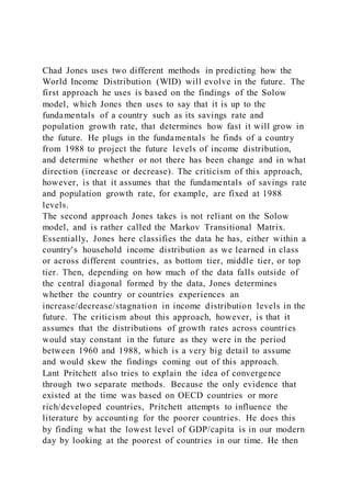
  • 57. lower bound on income (Pritchett and Summers, 1996). According to demographers, an under-five infant mortality rate of less than 600 per 1000 is necessary for a stable population (Hill, 1995). Using a regression based on Maddison's (1991) historical per capita income estimates and infant mortality data from historical sources for 22 countries, I predict that infant mortality in 1870 for a country with income of J$250 would have been 765 per 10O.9 Although the rate of natural increase of population back in 1870 is subject to great uncertainty, it is typically estimated to be between .25 and 1 percent annually in that period, which is again inconsistent with income levels as low as J$250.1o Divergence, Big Time If you accept: a) the current estimates of relative incomes across nations; b) the estimates of the historical growth rates of the now-rich nations; and c) that even in the poorest economies incomes were not below J$250 at any point-then you cannot escape the conclusion that the last 150 years have seen divergence, big time. The logic is straightforward and is well illustrated by Figure 1. If there had been no divergence, then we could extrapolate backward from present income of the poorer countries to past income assuming they grew at least as fast as the United
  • 58. 'The regression is estimated with country fixed effects: ln(IMR) = -.59 ln(GDP per capita) _ .013*Trend _ .002*Trend*(l if >1960) (23.7) (32.4) (14.23) N = 1994 and t-statistics are in parenthesis. The prediction used the average country constant of 9.91. "' Livi-Basci (1992) reports estimates of population growth in Africa between 1850 and 1900 to be .87 percent, and .93 percent between 1900 and 1950, while growth for Asia is estimated to be .27 1850 to 1900, and .61 1900 to 1950. Clark (1977) estimates the population growth rates between 1850 and 1900 to be .43 percent in Africa and India and lower, .33 percent, in China. 10 Journal of Economic Perspectives Figure 1 Simulation of Divergence of Per Capita GDP, 1870-1985 (showing only selected countries) 1870 1960 1990 Richest / poorest 8.7 38.5 45.2 std. dev.: 0.64 0.88 1.06 o | l j~~~~~~~~~~~~~~P$18054 USA USA - - -Ethiopia
  • 59. < <5 ..... Chad 90 - -- MirlimumI ct 00 W P$20631 1 ~~~~~~~~~~~Actual l X _ l ~~~~~~~~Imputed ll = _ l *-- | l ~~~~~~~~~~Chad P$250 (assumed lower bound) I l t ,,,, I,,,,,,,,,~~~~~~~~~ ~~~~ I, , I, , I, ,1,,, I . 1850 1870 1890 1910 1930 1950 1970 1990 2010 States. However, this would imply that many poor countries must have had incomes below J$100 in 1870. Since this cannot be true, there must have been divergence. Or equivalently, per capita income in the United States, the world's richest indus- trial country, grew about four-fold from 1870 to 1960. Thus, any country whose income was not fourfold higher in 1960 than it was in 1870 grew more slowly than the United States. Since 42 of the 125 countries in the Penn World Tables with data for 1960 have levels of per capita incomes below $1,000 (that is, less than four times
  • 60. $250), there must have been substantial divergence between the top and bottom. The figure of J$250 is not meant to be precise or literal and the conclusion of massive divergence is robust to any plausible assumption about a lower bound. Consider some illustrative calculations of the divergence in per capita incomes in Table 2. I scale incomes back from 1960 such that the poorest country in 1960 just reaches the lower bound by 1870, the leader in 1960 (the United States) reaches its actual 1870 value, and all relative rankings between the poorest country and the United States are preserved." The first row shows the actual path of the U.S. econ- " The growth rate of the poorest country was imposed to reach F$250 at exactly 1870, and the rate of the United States was used for the growth at the top. Then each country's growth rate was assumed to be a weighted average of those two rates, where the weights depended on the scaled distance from the bottom country in the beginning period of the imputation, 1960. This technique "smushes" the distri- Divergence, Big Time 11 Table 2 Estimates of the Divergence of Per Capita Incomes Since 1870 1870 1960 1990
  • 61. USA (F$) 2063 9895 18054 Poorest (F$) 250 257 399 (assumption) (Ethiopia) (Chad) Ratio of GDP per capita of richest to poorest country 8.7 38.5 45.2 Average of seventeen "advanced capitalist" countries 1757 6689 14845 from Maddison (1995) Average LDCs from PWT5.6 for 1960, 1990 (imputed for 740 1579 3296 1870) Average "advanced capitalist" to average of all other 2.4 4.2 4.5 countries Standard deviation of natural log of per capita incomes .51 .88 1.06 Standard deviation of per capita incomes F$459 F$2,112 F$3,988 Average absolute income deficit from the leader F$1286 F$7650 F$12,662 Notes: The estimates in the columns for 1870 are based on backcasting GDP per capita for each country using the methods described in the text assuming a minimum of P$250. If instead of that method, incomes in 1870 are backcast with truncation at P$250, the 1870 standard deviation is .64 (as reported in Figure 1). omy. The second row gives the level of the poorest economy in 1870, which is J$250 by assumption, and then the poorest economies in 1960 and 1990 taken from the
  • 62. Penn World Tables. By division, the third row then shows that the ratio of the top to the bottom income countries has increased from 8.7 in 1870 to 38 by 1960 and to 45 by 1990. If instead one takes the 17 richest countries (those shown in Table 1) and applies the same procedure, their average per capita income is shown in the fourth row. The average for all less developed economies appearing in the Penn World Tables for 1960 and 1990 is given in the fifth row; the figure for 1870 is calculated by the "backcasting" imputation process for historical incomes de- scribed above. By division, the sixth row shows that the ratio of income of the richest to all other countries has almost doubled from 2.4 in 1870 to 4.6 by 1990. bution back into the smaller range between the top and bottom while maintaining all cross country rankings. The formula for estimating the log of GDP per capita (GDPPC) in the ith country in 1870 was GDPPCi 870' = GDPPCi 96"* *(1/w,) where the scaling weight wi was wi = (1 - ai)*min(GDPPC'96()/F$250 + ai*GDPPCusA/GDPPCusA, and where ai is defined by ai = (GDPPC19N - min (S DPPC'9"))/(GDPPCL9? - min(CDPPC'96"()).
  • 63. 12 Journal of Economic Perspectives The magnitude of the change in the absolute gaps in per capita incomes between rich and poor is staggering. From 1870 to 1990, the average absolute gap in incomes of all countries from the leader had grown by an order of magnitude, from $1,286 to $12,662, as shown in the last row of Table 2.12 While the growth experience of all countries is equally interesting, some are more equally interesting than others. China and India account for more than a third of the world's population. For the conclusion of divergence presented here, however, a focus on India and China does not change the historical story. One can estimate their growth rates either by assuming that they were at $250 in 1870 and then calculating their growth rate in per capita GDP to reach the levels given by the Penn World Tables in 1960 (India, $766; China, $567), or by using Maddison's historical estimates, which are shown in Table 3, India's growth rate is a fifth and China's a third of the average for developed economies. Either way, India's and China's incomes diverged significantly relative to the leaders between 1870 and 1960. The idea that there is some lower bound to GDP per capita and that the lower
  • 64. bound has implications for long-run growth rates (and hence divergence) will not come as news either to economic historians or to recent thinkers in the area of economic growth (Lucas, 1996). Kuznets (1966, 1971) pointed out that since the now-industrialized countries have risen from very low levels of output to their pres- ently high levels, and that their previously very low levels of output were only con- sistent with a very slow rate of growth historically, growth rates obviously accelerated at some point. Moreover, one suspects that many of the estimates of income into the far distant past cited above rely on exactly this kind of counterfactual logic. Considering Alternate Sources of Historical Data Although there is not a great deal of historical evidence on GDP estimates in the very long-run for the less developed countries, what there is confirms the finding of massive divergence. Maddison (1995) reports time series data on GDP per capita incomes for 56 countries. These include his 17 "advanced capitalist" countries (presented in Table 1), five "southern" European countries, seven eastern Euro- pean countries and 28 countries typically classified as "less developed" from Asia (11), Africa (10) and Latin America (7). This data is clearly nonrepresentative of the poorest countries (although it does include India and China), and the data for Africa is very sparse until 1960. Even so, the figures in Table 3
  • 65. show substantially lower growth for the less developed countries than for the developed countries. If 12 In terms of standard deviations, the method described in the text implies that the standard deviation of the national log of per capita GDP has more than doubled from 1870 to 1990, rising from .51 in 1870 to .88 in 1960 to 1.06 by 1990. In dollar terms, the standard deviation of per capita incomes rose from $459 in 1870 to $2,112 in 1960 to $3,988 in 1990 (again, all figures expressed in 1985 dollars, converted at purchasing power equivalent exchange rates). Lant Pritchett 13 Table 3 Mean Per Annum Growth Rates of GDP Per Capita 1870-1960 1960-1979 1980-1994 Advanced capitalist countries (17) 1.5 3.2 1.5 (.33) (1.1) (.51) Less developed countries (28) 1.2 2.5 .34 (.88) (1.7) (3.0) Individual countries: India .31 1.22 3.07 China .58 2.58 6.45 Korea (1900) .71 5.9 7.7 Brazil 1.28 4.13 -.54 Argentina (1900) 1.17 1.99 .11 Egypt (1900) .56 3.73 2.21
  • 66. Source: Calculations based on data from Maddison (1995). one assumes that the ratio of incomes between the "advanced capitalist" countries and less developed countries was 2.4 in 1870, then the .35 percentage point differ- ential would have produced a rich-poor gap of 3.7 in 1994, similar to the projected increase in the gap to 4.5 in Table 2. Others have argued that incomes of the developing relative to the developed world were even higher in the past. Hanson (1988, 1991) argues that adjustments of comparisons from official exchange rates to purchasing power equivalents imply that developing countries were considerably richer historically than previously be- lieved. Bairoch (1993) argues that there was almost no gap between the now- developed countries and the developing countries as late as 1800. As a result, his estimate of the growth rate of the "developed" world is 1.5 percent between 1870 and 1960 as opposed to .5 percent for the "developing" world, which implies even larger divergence in per capita incomes than the lower bound assumptions reported above. Poverty Traps, Takeoffs and Convergence The data on growth in less developed countries show a variety of experiences, but divergence is not a thing of the past. Some countries are
  • 67. "catching up" with very explosive but sustained bursts of growth, some countries continue to experi- ence slower growth than the richest countries, and others have recently taken nosedives. Let's set the standard for explosive growth in per capita GDP at a sustained rate of 4.2 percent; this is the fastest a country could have possibly grown from 1870 to 1960, as at this rate a country would have gone from the lower bound in 1870 14 Journal of Economic Perspectives to the U.S. level in 1960. Of the 108 developing countries for which there are available data in the Penn World Tables, 11 grew faster than 4.2 per annum over the 1960-1990 period. Prominent among these are east Asian economies like Korea (6.9 percent annual growth rate in per capita GDP from 1960- 1992), Taiwan (6.3 percent annual growth) and Indonesia (4.4 percent). These countries are growing at an historically unprecedented pace. However, many countries that were poor in 1960 continued to stagnate. Sixteen developing countries had negative growth over the 1960-1990 period, including Mozambique (-2.2 percent per annum) and Guy- ana (-.7 percent per annum). Another 28 nations, more than a quarter of the total
  • 68. number of countries for which the Penn World Tables offers data, had growth rates of per capita GDP less than .5 percent per annum from 1960 to 1990 (for example, Peru with .1 percent); and 40 developing nations, more than a third of the sample, had growth rates less than 1 percent per annum.'3 Moreover, as Ben-David and Papell (1995) emphasize, many developing coun- tries have seen their economies go into not just a slowdown, but a "meltdown." If we calculate the growth rates in the Penn World Tables and allow the data to dictate one break in the growth rate over the whole 1960-1990 period, then of the 103 developing countries, 81 have seen a deceleration of growth over the period, and the average deceleration is over 3 percentage points. From 1980-1994, growth in per capita GDP averaged 1.5 percent in the advanced countries and .34 percent in the less developed countries. There has been no acceleration of growth in most poor countries, either absolutely or relatively, and there is no obvious reversal in divergence. These facts about growth in less developed countries highlight its enormous vari- ability and volatility. The range of annual growth rates in per capita GDP across less developed economies from 1960 to 1990 is from -2.7 percent to positive 6.9 percent. Taken together, these findings imply that almost nothing that is
  • 69. true about the growth rates of advanced countries is true of the developing countries, either in- dividually or on average. The growth rates for developed economies show conver- gence, but the growth rates between developed and developing economies show considerable divergence. The growth rates of developed countries are bunched in a narrow group, while the growth rates of less developed countries are all over with some in explosive growth and others in implosive decline. Conclusion For modem economists, Gerschenkron (1962) popularized the idea of an "ad- vantage to backwardness," which allows countries behind the technological frontier to 13 The division into developed and developing is made here by treating all 22 high-income members of the OECD as "developed" and all others as "developing." Divergence, Big Time 15 experience episodes of rapid growth driven by rapid productivity catch-up.'4 Such rapid gains in productivity are certainly a possibility, and there have been episodes of indi- vidual countries with very rapid growth. Moreover, there are examples of convergence in incomes amongst regions. However, the prevalence of absolute divergence implies
  • 70. that while there may be a potential advantage to backwardness, the cases in which backward countries, and especially the most backward of countries, actually gain sig- nificantly on the leader are historically rare. In poor countries there are clearly forces that create the potential for explosive growth, such as those witnessed in some countries in east Asia. But there are also strong forces for stagnation: a quarter of the 60 countries with initial per capita GDP of less than $1000 in 1960 have had growth rates less than zero, and a third have had growth rates less than .05 percent. There are also forces for "implosive" decline, such as that witnessed in some countries in which the fabric of civic society appears to have disintegrated altogether, a point often ignored or ac- knowledged offhand as these countries fail to gather plausible economic statistics and thus drop out of our samples altogether. Backwardness seems to carry severe disadvan- tages. For economists and social scientists, a coherent model of how to overcome these disadvantages is a pressing challenge. But this challenge is almost certainly not the same as deriving a single "growth theory." Any theory that seeks to unify the world's experience with economic growth and development must address at least four distinct questions: What accounts for con- tinued per capita growth and technological progress of those leading countries at the frontier? What accounts for the few countries that are able to initiate and sustain
  • 71. periods of rapid growth in which they gain significantly on the leaders? What accounts for why some countries fade and lose the momentum of rapid growth? What accounts for why some countries remain in low growth for very long periods? Theorizing about economic growth and its relation to policy needs to tackle these four important and distinct questions. While it is conceivable that there is an all- purpose universal theory and set of policies that would be good for promoting eco- nomic growth, it seems much more plausible that the appropriate growth policy will differ according to the situation. Are we asking about more rapid growth in a mature and stable economic leader like the United States or Germany or Japan? About a booming rapidly industrializing economy trying to prevent stalling on a plateau, like Korea, Indonesia, or Chile? About a once rapidly growing and at least semi- industrialized country trying to initiate another episode of rapid growth, like Brazil or Mexico or the Philippines? About a country still trying to escape a poverty trap into sustained growth, like Tanzania or Myanmar or Haiti? Discussion of the theory and policy of economic growth seems at times remarkably insensitive to these distinctions. * I would like to thank William Easterly, Deon Filmer, Jonathan Isham, Estelle James, Ross Levine, Mead Over, Martin Rama and Martin Ravallion for helpful discussions and comments.
  • 72. '4 I say "for modern economists," since according to Rostow (1993), David Hume more than 200 years ago argued that the accumulated technological advances in the leading countries would give the followers an advantage. 16 Journal of Economic Perspectives References Bairoch, Paul, Economics and World History: Myths and Paradoxes. Chicago: University of Chi- cago Press, 1993. Barro, Robert, "Economic Growth in a Cross Section of Countries," QuarterlyJournal ofEconom- ics, May 1991, 106, 407-43. Barro, Robert, and Xavier Sala-i-Martin, " Con- vergence, " Journal of PoliticalEconomy, April 1992, 100, 223-51. Barro, Robert, and Xavier Sala-i-Martin, Eco- nomic Growth. New York: McGraw Hill, 1995. Baumol, Wiam, "Productivity Growth, Con- vergence and Welfare: What the Long-Run Data Show," American Economic Review, December 1986, 76, 1072-85. Ben-David, Dan, "Equalizing Exchange: Trade Liberalization and Convergence," QuarterlyJour- nal of Economics, 1993, 108:3, 653-79.
  • 73. Ben-David, Dan, and David Papeli, "Slow- downs and Meltdowns: Post-War Growth Evi- dence from 74 countries." Centre for Economic Policy Research Discussion Paper Series No. 1111, February 1995. Canova, Fabio, and Albert Marcet, "The Poor Stay Poor: Non-Convergence Across Countries and Regions." Centre for Economic Policy Re- search Discussion Paper No. 1265, November 1995. Caselli, Franseco, Gerardo Esquivel, and Fer- nando Lefort, "Reopening the Convergence De- bate: A New Look at Cross-Country Growth Em- pirics," mimeo, Harvard University, 1995. Chen, Shaohua, Gaurav Datt, and Martin Ra- vallion, "Is Poverty Increasing in the Developing World?" World Bank Policy Research Working Paper No. 1146, June 1993. Clark, Colin, Population Growth and Land Use. London: Macmillan, 1977. De Long, Bradford, "Productivity Growth, Convergence, and Welfare: Comment," American Economic Review, December 1988, 78, 1138-54. Dollar, David, and Edward Wolff, Competitive- ness, Convergence, and International Specialization. Cambridge, Mass.: Massachusetts Institute of Technology Press, 1993. Easterly, William, Michael Kremer, Lant
  • 74. Pritchett, and Lawrence Summers, "Good Policy or Good Luck? Country Growth Performance and Temporary Shocks," Journal of Monetary Eco- nomics, December 1993, 32:3, 459-83. Evans, Paul, "Evaluating Growth Theories Us- ing Panel Data," mimeo, Ohio State University, 1994. de la Fuente, Angel, "The Empirics of Growth and Convergence: A Selective Review." Centre for Economic Policy Research No. 1275, Novem- ber 1995. FAO, Calorie Requirements: Report of the Second Committee on Calorie Requirements. Rome: FAO, 1957. FAO, Handbook on Human Nutritional Require- ments. Rome: Food and Agriculture Organization and World Health Organization, 1974. Gerschenkron, Alexander, Economic Backward- ness in Historical Perspective, a Book of Essays. Cam- bridge: Belknap Press, 1962. Hanson, John R., "Third World Incomes be- fore World War I: Some Comparisons," Explora- tions in Economic History, 1988, 25, 323-36. Hanson, John R., "Third World Incomes be- fore World War I: Further Evidence," Explora- tions in Economic History, 1991, 28, 367-79. Hill, Kenneth, "The Decline of Childhood
  • 75. Mortality." In Simon, Julian, ed., The State of Hu- manity. Oxford: Blackwell, 1995, pp. 37-50. International Rice Research Institute, World Rice Statistics. Los Banos: International Rice Re- search Institute, 1987. Jones, Charles, "R&D Based Models of Eco- nomic Growth," Journal of Political Economy, Au- gust 1995, 103:4, 759-84. Kuznets, Simon, Modern Economic Growth: Rate, Structure and Spread. New Haven: Yale University Press, 1966. Kuznets, Simon, Economic Growth of Nations: To- tal Output and Production Structure. Cambridge, Mass.: Belknap Press, 1971. Livi-Basci, Massimo, A Concise History of World Population. Cambridge, Mass: Blackwell, 1992. Loayza, Norman, "A Test of the International Convergence Hypothesis Using Panel Data." World Bank Policy Research Paper No. 1333, Au- gust 1994. Lucas, Robert, "Ricardian Equilibrium: A Neoclassical Exposition," mimeo, Technion Is- rael Institute of Technology Economics Work- shop Series, June 1996. Maddison, Angus, "A Comparison of Levels of GDP Per Capita in Developed and Developing Countries, 1700-1980," Journal of Economic His- tory, March 1983, 43, 27-41.
  • 76. Maddison, Angus, Dynamic Forces in Capitalistic Development: A Long-Run Comparative View. New York: Oxford University Press, 1991. Maddison, Angus, "Explaining the Economic Performance of Nations, 1820-1989." In Bau- mol, William J., Richard R. Nelson, and Edward N. Wolff, eds., Convergence of Productivity: Cross- Lant Pritchett 17 National Studies and Historical Evidence. New York: Oxford University Press, 1994, pp. 20-61. Maddison, Angus, Monitoring the World Econ- omy, 1820-1992. Paris: Development Centre of the Organisation for Economic Co-operation De- velopment, 1995. Mankiw, N. Gregory, David Romer, and David Weil, "A Contribution to the Empirics of Eco- nomic Growth," Quarterly Journal of Economics, May 1992, 107:2, 407-36. Nuxoll, Daniel, "Differences in Relative Prices and International Differences in Growth Rates," American Economic Review, Decmeber 1994, 84, 1423-36. Pritchett, Lant, "Where Has All the Education Gone?," mimeo, June 1995a. Pritchett, Lant, "Population, Factor Accumu-
  • 77. lation and Productivity." World Bank Policy Re- search Paper No. 1567, October 1995b. Pritchett, Lant, and Lawence H. Summers, "Wealthier is Healthier," Journal of Human Re- sources, 1996, 31:4, 841-68. Quah, Danny, "Empirics for Economic Growth and Convergence." Centre for Eco- nomic Policy Research Discussion Paper No. 1140, March 1995. Ravallion, Martin, Gaurav Datt, and Domi- nique van de Walle, "Quantifying Absolute Pov- erty in the Developing World," Review of Income and Wealth, 1991, 37:4, 345-61. Rebelo, Sergio, "Long-Run PolicyAnalysis and Long-Run Growth," Journal of Political Economy, June 1991, 99, 500-21. Rostow, W. W., Theorist of Economic Growth from David Hume to the Present: With a Perspective on the Next Century. New York: Oxford University Press, 1990. Sachs, Jeffrey, and Andrew Warner, "Eco- nomic Convergence and Economic Policies." NBER Working Paper No. 5039, February 1995. Sala-i-Martin, Xavier, "Regional Cohesion: Ev- idence and Theories of Regional Growth and Convergence." Centre for Economic Policy Re- search Discussion Paper No. 1074, November 1994.
  • 78. Summers, Robert, and Alan Heston, "The Penn World Tables (Mark 5): An Expanded Set of International Comparisons, 1950-88," Quar- terly Journal of Economics, 1991, 106:2, 327-68. World Bank, World Development Report: Workers in an Integrating Economy. Washington, D.C.: Ox- ford University Press for the World Bank, 1995. Article Contentsp. [3]p. 4p. 5p. 6p. 7p. 8p. 9p. 10p. 11p. 12p. 13p. 14p. 15p. 16p. 17Issue Table of ContentsThe Journal of Economic Perspectives, Vol. 11, No. 3 (Summer, 1997), pp. 1- 202+i-viFront Matter [pp. 1 - 2]Symposium: Distribution of World IncomeDivergence, Big Time [pp. 3 - 17]On the Evolution of the World Income Distribution [pp. 19 - 36]Symposium: European UnemploymentLabor Market Rigidities: At the Root of Unemployment in Europe [pp. 37 - 54]Unemployment and Labor Market Rigidities: Europe versus North America [pp. 55 - 74]Symposium: Electronic Journals in EconomicsThe Future Information Infrastructure in Economics [pp. 75 - 94]The AEA's Electronic Publishing Plans: A Progress Report [pp. 95 - 104]Bridging the Gap Between the Public's and Economists' Views of the Economy [pp. 105 - 118]Restructuring, Competition and Regulatory Reform in the U.S. Electricity Sector [pp. 119 - 138]FDICIA After Five Years [pp. 139 - 158]A Nobel Prize for Game Theorists: The Contributions of Harsanyi, Nash and Selten [pp. 159 - 174]Policy Watch: The Family and Medical Leave Act [pp. 175 - 186]Recommendations for Further Reading [pp. 187 - 194]Correspondence [pp. 195 - 198]Notes [pp. 199 - 202]Back Matter [pp. i - vi]