mechanic and problems

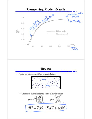
1. Comparing Model Results
μ = −T
∂S
∂N
⎛
⎝
⎜
⎞
⎠
⎟
U,V
μ =
∂U
∂N
⎛
⎝
⎜
⎞
⎠
⎟
S,V
dU = TdS − PdV + μdN
Review
• For two systems in diffusive equilibrium
– Chemical potential is the same at equilibrium

2. Chemical Potential
• Consider relation
μ =
∂U
∂N
⎛
⎝
⎜
⎞
⎠
⎟
S,V

3. Different Types of Particles
• Initially, we assumed only one type of particle in system
• If it contains several different types of particles
– Need to consider chemical potential for each one
– Thermodynamic identity becomes
μ1 ≡ −T
∂S
∂N1
⎛
⎝
⎜
⎞
⎠
⎟
U,V ,N2
μ2 =
∂U
∂N2
⎛
⎝
⎜
⎞
⎠
⎟
S,V ,N1
dU = TdS − PdV + μidNi
i
∑
More on Diffusive Equilibrium
• Now consider system in thermal equilibrium and diffusive
equilibrium with reservoir at temperature, T
– System can exchange particles with environment
• Ratio of probabilities for two different microstates
P(s2)
P(s1)
=
ΩR (s2)
ΩR (s1)

4. Gibbs Factor
• Starting from P(s2)
P(s1)
=
ΩR (s2)
ΩR (s1)
=
eSR (s2 )/ k
eSR (s1 )/ k
= e SR (s2 )−SR (s1 )
[ ]/k
Calculating Absolute Probabilities
• Normalizing function for Gibbs factor:
• Grand Partition Function (or Gibbs sum)
– Sum over all possible states (including all possible N)
• Gibbs factor for different types of particles (example two)
Z = e
− E (s)−μN (s)
[ ]/ kT
s
∑
e− E(s)−μA NA (s)−μB NB (s)
[ ]/kT

5. Stat Mech Terminology
• For isolated system (as in the ones just used),
– All microstates have same probability
– Microcannonical ensemble
• For system in thermal equilibrium with a reservoir at T,
– State probabilities determined from Boltzmann factors
– Cannonical ensemble
• For system in thermal and diffusive equilibrium with reservoir,
– State probabilities determined from Gibbs factors
– Grand cannonical ensemble
Quantum Statistics
• Useful application of Gibbs factors
• Consider an ideal gas
– Partition function derived for N indistinguishable, non-
interacting particles
– Number of single-particle states much greater than number
of particles
Ztotal =
1
N!
Z1
N
Z1 >> N

6. System of Non-interacting Particles
• Start with a system of two non-interacting particles that can
occupy any of five single-particle states
• Each single particle state has E=0 so each Boltzmann factor is
1 so Z is same as Ω
11000 01010 20000
10100 01001 02000
10010 00110 00200
10001 00101 00020
01100 00011 00002
• If distinguishable particles, Z=25
• If indistinguishable particles, Z=15 - not Boltzmann value
Distribution Functions
• If Z1>>N not valid, can use Gibbs factors instead of Boltzmann
factors
– Need to consider if particles are bosons or fermions
• Start with one single-particle state of system,
– Energy when occupied is ε, when unoccupied is 0
– If can be occupied by n particles, probability is
P(n) =
1
Ζ
e−(nε−μn)/ kT
=
1
Ζ
e−n(ε−μ)/ kT

7. Fermi-Dirac Distribution
• For a fermion,
– n can either be 0 or 1
– So grand partition function is
– Average number of particles in state (its occupancy)
Z =1+ e−(ε−μ)/ kT
n = nP(n)
n
∑ =
e−(ε−μ)/ kT
1+ e−(ε−μ)/ kT
nFD =
1
e(ε−μ)/ kT
+1
Bose-Einstein Distribution
• For a boson,
– n can be any non-negative integer
– So grand partition function is
– Average number of particles in state (its occupancy)
Z =1+ e−(ε−μ)/ kT
+ e−2(ε−μ)/ kT
+K
=
1
1− e−(ε−μ)/ kT
n = nP(n)
n
∑