sorting, daa

1. Quick Sort
Quicksort Concept
(<pivot)
LEFT group
(> pivot)
RIGHT group
apply Quicksort to the subgroups

2. Quick Sort
Quicksort Start
Unsorted Array

3. Quick Sort
Quicksort Step 1
pivot
26 33 35 29 19 12 22

4. Quick Sort
left
Quicksort Step 2
pivot
26 33 35 29 19 12 22
right

5. Quick Sort
left
Quicksort Step 3
pivot
26 33 35 29 19 12 22
right

6. Quick Sort
left
Quicksort Step 4
pivot
26 33 35 29 19 12 22
right
left
pivot
26 22 35 29 19 12 33
right

7. Quick Sort
left
26 22 35 29 19
left
Quicksort Step 5
pivot
12 33
right

8. Quick Sort
left
26 22 35 29 19 12 33
right
pivot
26 22 12 29 19 35 33
left right
Quicksort Step 6
pivot

9. Quick Sort
26 22 12 29 19
left
Quicksort Step 7
pivot
35 33
right
pivot
26 22 12 19 29 35 33
right left

10. Quick Sort
26 22 12 19 29 35 33
26
19 22 12 29
Quicksort Step 8
pivot
right left
pivot
35
LEFT RIGHT

11. Quick Sort
26
19 22 12
Quicksort Step 9
previous pivot
29 35 33
Quicksort Quicksort
pivot pivot
12 19 22 29 33 35
26
12 19 22 26 29 33 35

12. Quick Sort
Quicksort Efficiency

13. Quick Sort






Best Case

14. Quick Sort



Worst case

15. Quick Sort





Worst case for quicksort

16. 16
Sorting
• Selection sort
– Design
approach:
– Sorts in place:
– Running time:
• Merge Sort
– Design
approach:
– Sorts in place:
– Running time:
incrementa
l
Yes
(n2)
divide and
conquer No
Let’s see!!

17. 1
7
Divide-and-Conquer
• Divide the problem into a number of sub-
problems
– Similar sub-problems of smaller size
• Conquer the sub-problems
– Solve the sub-problems recursively
– Sub-problem size small enough  solve the
problems in straightforward manner
• Combine the solutions of the sub-problems
– Obtain the solution for the original problem

18. 1
8
Merge Sort Approach
• To sort an array A[p . . r]:
• Divide
– Divide the n-element sequence to be sorted into
two subsequences of n/2 elements each
• Conquer
– Sort the subsequences recursively using merge
sort
– When the size of the sequences is 1 there is
nothing more to do
• Combine
– Merge the two sorted subsequences

19. Merge Sort
p
Alg.: MERGE-SORT(A, p,
r)
if p < r
then q ← (p + r)/2
MERGE-SORT(A, p, q)
MERGE-SORT(A, q +
1, r) MERGE(A, p, q,
r)
Check for base
case
Divid
e
Conque
r
Conque
r
Combin
e
• Initial call: MERGE-SORT(A,
1, n)
1 2 3 4 5 6 7 8
5 2 4 7 1 3 2 6
r
q
1
9

20. Example – n Power of2
1 2 3 4 5 6 7 8
q =
4
5 2 4 7 1 3 2 6
1 2 3 4
5 2 4 7
5 6 7 8
1 3 2 6
1 2
2
5
3 4
7
4
5 6
3
1
7 8
6
2
1 2 3 4 5 6 7 8
5 2 4 7 1 3 2 6
Divid
e
20

21. Example – n Power of2
1 2 3 4 5 6 7 8
5 2 4 7 1 3 2 6
1 2 3 4 5 6 7 8
1 2 2 3 4 5 6 7
1 2 3 4
2 4 5 7
5 6 7 8
1 2 3 6
1 2
5
2
3 4
7
4
5 6
3
1
7 8
6
2
Conque
r and
Merge
21

22. Example – n Not a Power of2
4 7 2 6 1 4 7 3 5 2 6
1 2 3 4 5 6 7 8 9 10 11
q =
6
4 7 2 6 1 4
1 2 3 4 5 6
7 3 5 2 6
7 8 9 10 11
q =
9
q =
3
4 7 2
1 2 3
6 1 4
4 5 6
7 3 5
7 8 9
6
2
10 11
7
4
1 2
2
3
1
6
4 5
4
6
3
7
7 8
5
9
2
10
6
11
4
1
7
2
6
4
1
5
7
7
3
8
Divid
e
22

23. Example – n Not a Power of2
1 2 2 3 4 4 5 6 6 7 7
1 2 3 4 5 6 7 8 9 10 11
1 2 4 4 6 7
1 2 3 4 5 6
2 3 5 6 7
7 8 9 10 11
2 4 7
1 2 3
1 4 6
4 5 6
3 5 7
7 8 9
6
2
10 11
2
3
4
6
5
9
2
10
6
11
4
1
7
2
6
4
1
5
7
7
3
8
4 7
1 2
6
1
4 5
7
3
7 8
Conque
r and
Merge
23

24. 11
Merge - Pseudocp
ode
Alg.: MERGE(A, p,
q, r)
1. Compute n1 and
n2
2. Copy the first n1 elements
into
. . n1 + 1] and the next n2 elements into R[1 . . n2 +
1]
3. L[n1 + 1] ← ; R[n2 + 1] ←
4. i ← 1; j ← 1
5. for k ← p to
r
6. do if L[ i ] ≤ R[ j ]
7. then A[k] ← L[ i
]
8. i ←i + 1
9. else A[k] ← R[ j
]
p q
2 4 5 7 
1 2 3 6 
r
q +
1
L
R
1 2 3 4 5 6 7 8
2 4 5 7 1 2 3 6
r
q
Ln2
[1
n1

25. Algorithm:
mergesort( int [] a, int left, int right)
{
if (right > left)
{ middle = left + (right -
left)/2; mergesort(a, left,
middle); mergesort(a,
middle+1, right); merge(a,
left, middle, right); }
}
Complexity of Merge
Sort

26. 1
4
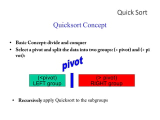
Quicksort
A[p…q]
• Sort an array A[p…r]
• Divide
– Partition the array A into 2 subarrays A[p..q] and A[q+1..r],
such that each element of A[p..q] is smaller than or equal to
each element in A[q+1..r]
– Need to find index q to partition the array
≤ A[q+1…r]

27. Quicksort
A[p…q]
• Conquer
– Recursively sort A[p..q] and A[q+1..r]using
Quicksort
• Combine
– Trivial: the arrays are sorted in place
– No additional work is required to combine them
– The entire array is now sorted
A[q+1…r]
≤
27

28. 28
Recurrence
Initially: p=1, r=n
Alg.: QUICKSORT(A, p, r)
if p < r
then q  PARTITION(A, p,
r) QUICKSORT (A,
p, q) QUICKSORT
(A, q+1, r)
Recurrence:

29. Partitioning the Array
Alg. PARTITION (A,
p, r)
1. x  A[p]
2. i  p – 1
3. j  r + 1
4. while TRUE
5. do repeat j  j –
1
6. until A[j] ≤ x
7. do repeat i  i +
1
8. until A[i] ≥ x
9. if i < j
then exchange A[i] 
A[j]
else return j
Each element
is visited
once!
Running time:
(n) n = r – p + 1
5 3 2 6 4 1 3 7
i j
A
:
ap ar
j=q i
A
:
A[p…q]
29
A[q+1…r]
≤
p r

30. Partition can be done in O(n) time, where n is the
size of the array. Let T(n) be the number of
comparisons required by Quicksort.
If the pivot ends up at position k, then we have
T(n) T(nk)  T(k 1)  n
To determine best-, worst-, and average-case
complexity
we need to determine the values of k that
correspond to these cases.
Analysis of quicksort

31. Master Theorem Merge Sort Example
• Recurrence relation:
T(n) = 2T(n/2) + O(n)
• Variables:
a = 2
b = 2
f(n) = O(n)
• Comparison:
nlog
b
(a) <=> O(n)
n1 == O(n)
• Here we see that the cost of f(n) and the subproblems are the same,
so this is Case 2:
T(n) = O(nlogn)

32. Master theorum
T(n) = aT(n/b) + f(n)
where,
T(n) has the following asymptotic bounds:
1. If f(n) = O(nlog
b
a-ϵ), then T(n) = Θ(nlog
b
a).
2. 2. If f(n) = Θ(nlog
b
a), then T(n) = Θ(nlog
b
a * log n).
3. 3. If f(n) = Ω(nlog
b
a+ϵ), then T(n) = Θ(f(n)). ϵ > 0 is a constant.

33. Quick sort Complexity worst case
• QUICKSORT
Worst Case Analysis
Recurrence Relation:
T(0) = T(1) = 0 (base case)
T(N) = N + T(N-1)
Solving the RR:
T(N) = N + T(N-1)
T(N-1) = (N-1) + T(N-2)
T(N-2) = (N-2) + T(N-3)
...
T(3) = 3 + T(2)
T(2) = 2 + T(1)
T(1) = 0
Hence,
T(N) = N + (N-1) + (N-2) ... + 3 + 2
≈ N 2
2
which is O(N 2 )