Download as PDF, PPTX


![12/43
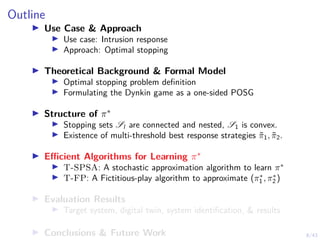
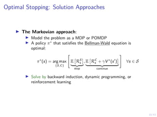
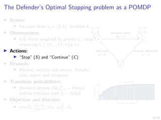
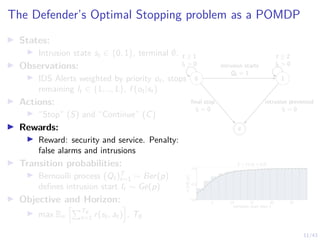
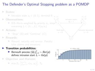
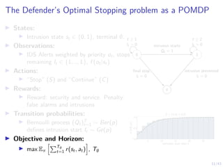
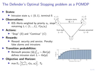
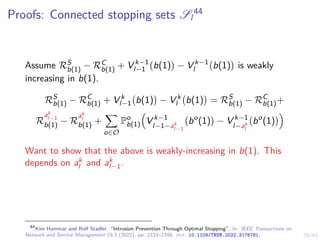
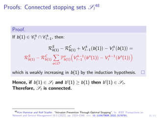
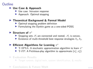
The Attacker’s Optimal Stopping problem as an MDP
I States:
I Intrusion state st ∈ {0, 1}, terminal ∅,
defender belief b ∈ [0, 1].
I Actions:
I “Stop” (S) and “Continue” (C)
I Rewards:
I Reward: denial of service and intrusion.
Penalty: detection
I Transition probabilities:
I Intrusion starts and ends when the
attacker takes stop actions
I Objective and Horizon:
I max Eπ
hPT∅
t=1 r(st, at)
i
, T∅
0 1
∅
t ≥ 1 t ≥ 2
intrusion starts
at = 1
final stop detected](https://image.slidesharecdn.com/nyuinvitedtalkoptimalstoppinghammar30jan-230130171136-e7c97858/85/Intrusion-Response-through-Optimal-Stopping-47-320.jpg)

![15/43
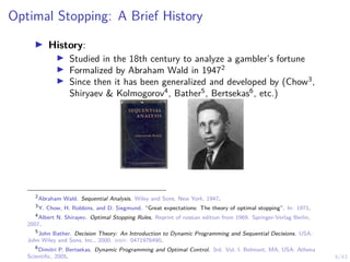
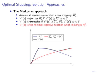
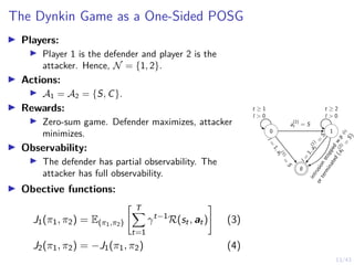
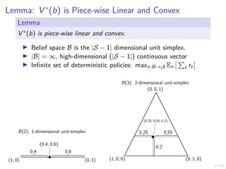
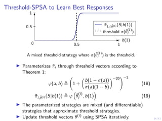
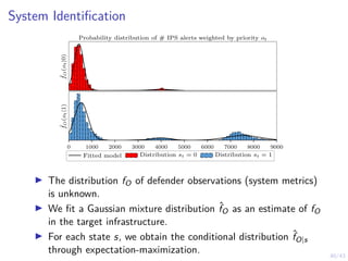
Structural Result: Optimal Multi-Threshold Policy
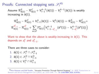
Theorem
Given the intrusion response POMDP, the following holds:
1. Sl−1 ⊆ Sl for l = 2, . . . L.
2. If L = 1, there exists an optimal threshold α∗ ∈ [0, 1] and an
optimal defender policy of the form:
π∗
L(b(1)) = S ⇐⇒ b(1) ≥ α∗
(5)
3. If L ≥ 1 and fX is totally positive of order 2 (TP2), there
exists L optimal thresholds α∗
l ∈ [0, 1] and an optimal
defender policy of the form:
π∗
l (b(1)) = S ⇐⇒ b(1) ≥ α∗
l , l = 1, . . . , L (6)
where α∗
l is decreasing in l.](https://image.slidesharecdn.com/nyuinvitedtalkoptimalstoppinghammar30jan-230130171136-e7c97858/85/Intrusion-Response-through-Optimal-Stopping-50-320.jpg)
![15/43
Structural Result: Optimal Multi-Threshold Policy
Theorem
Given the intrusion response POMDP, the following holds:
1. Sl−1 ⊆ Sl for l = 2, . . . L.
2. If L = 1, there exists an optimal threshold α∗ ∈ [0, 1] and an
optimal defender policy of the form:
π∗
L(b(1)) = S ⇐⇒ b(1) ≥ α∗
(7)
3. If L ≥ 1 and fX is totally positive of order 2 (TP2), there
exists L optimal thresholds α∗
l ∈ [0, 1] and an optimal
defender policy of the form:
π∗
l (b(1)) = S ⇐⇒ b(1) ≥ α∗
l , l = 1, . . . , L (8)
where α∗
l is decreasing in l.](https://image.slidesharecdn.com/nyuinvitedtalkoptimalstoppinghammar30jan-230130171136-e7c97858/85/Intrusion-Response-through-Optimal-Stopping-51-320.jpg)
![15/43
Structural Result: Optimal Multi-Threshold Policy
Theorem
Given the intrusion response POMDP, the following holds:
1. Sl−1 ⊆ Sl for l = 2, . . . L.
2. If L = 1, there exists an optimal threshold α∗ ∈ [0, 1] and an
optimal defender policy of the form:
π∗
L(b(1)) = S ⇐⇒ b(1) ≥ α∗
(9)
3. If L ≥ 1 and fX is totally positive of order 2 (TP2), there
exists L optimal thresholds α∗
l ∈ [0, 1] and an optimal
defender policy of the form:
π∗
l (b(1)) = S ⇐⇒ b(1) ≥ α∗
l , l = 1, . . . , L (10)
where α∗
l is decreasing in l.](https://image.slidesharecdn.com/nyuinvitedtalkoptimalstoppinghammar30jan-230130171136-e7c97858/85/Intrusion-Response-through-Optimal-Stopping-52-320.jpg)
![15/43
Structural Result: Optimal Multi-Threshold Policy
Theorem
Given the intrusion response POMDP, the following holds:
1. Sl−1 ⊆ Sl for l = 2, . . . L.
2. If L = 1, there exists an optimal threshold α∗ ∈ [0, 1] and an
optimal defender policy of the form:
π∗
L(b(1)) = S ⇐⇒ b(1) ≥ α∗
(11)
3. If L ≥ 1 and fX is totally positive of order 2 (TP2), there
exists L optimal thresholds α∗
l ∈ [0, 1] and an optimal
defender policy of the form:
π∗
l (b(1)) = S ⇐⇒ b(1) ≥ α∗
l , l = 1, . . . , L (12)
where α∗
l is decreasing in l.](https://image.slidesharecdn.com/nyuinvitedtalkoptimalstoppinghammar30jan-230130171136-e7c97858/85/Intrusion-Response-through-Optimal-Stopping-53-320.jpg)
![16/43
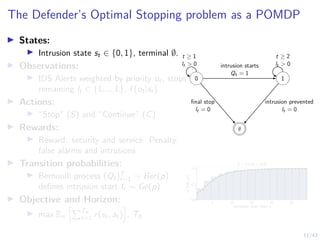
Structural Result: Optimal Multi-Threshold Policy
b(1)
0 1
belief space B = [0, 1]](https://image.slidesharecdn.com/nyuinvitedtalkoptimalstoppinghammar30jan-230130171136-e7c97858/85/Intrusion-Response-through-Optimal-Stopping-54-320.jpg)
![16/43
Structural Result: Optimal Multi-Threshold Policy
b(1)
0 1
belief space B = [0, 1]
S1
α∗
1](https://image.slidesharecdn.com/nyuinvitedtalkoptimalstoppinghammar30jan-230130171136-e7c97858/85/Intrusion-Response-through-Optimal-Stopping-55-320.jpg)
![16/43
Structural Result: Optimal Multi-Threshold Policy
b(1)
0 1
belief space B = [0, 1]
S1
S2
α∗
1
α∗
2](https://image.slidesharecdn.com/nyuinvitedtalkoptimalstoppinghammar30jan-230130171136-e7c97858/85/Intrusion-Response-through-Optimal-Stopping-56-320.jpg)
![16/43
Structural Result: Optimal Multi-Threshold Policy
b(1)
0 1
belief space B = [0, 1]
S1
S2
.
.
.
SL
α∗
1
α∗
2
α∗
L
. . .](https://image.slidesharecdn.com/nyuinvitedtalkoptimalstoppinghammar30jan-230130171136-e7c97858/85/Intrusion-Response-through-Optimal-Stopping-57-320.jpg)

![19/43
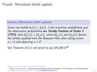
Proofs: S1 is convex10
I S1 is convex if:
I for any two belief states b1, b2 ∈ S1
I any convex combination of b1, b2 is also in S1
I i.e. b1, b2 ∈ S1 =⇒ λb1 + (1 − λ)b2 ∈ S1 for λ ∈ [0, 1].
I Since V ∗(b) is convex:
V ∗
(λb1 + (1 − λ)b2) ≤ λV ∗
(b1) + (1 − λ)V (b2)
I Since b1, b2 ∈ S1:
V ∗
(b1) = Q∗
(b1, S) S=stop
V ∗
(b2) = Q∗
(b2, S) S=stop
10
Vikram Krishnamurthy. Partially Observed Markov Decision Processes: From Filtering to Controlled Sensing.
Cambridge University Press, 2016. doi: 10.1017/CBO9781316471104.](https://image.slidesharecdn.com/nyuinvitedtalkoptimalstoppinghammar30jan-230130171136-e7c97858/85/Intrusion-Response-through-Optimal-Stopping-63-320.jpg)
![19/43
Proofs: S1 is convex11
I S1 is convex if:
I for any two belief states b1, b2 ∈ S1
I any convex combination of b1, b2 is also in S1
I i.e. b1, b2 ∈ S1 =⇒ λb1 + (1 − λ)b2 ∈ S1 for λ ∈ [0, 1].
I Since V ∗(b) is convex:
V ∗
(λb1 + (1 − λ)b2) ≤ λV ∗
(b1) + (1 − λ)V (b2)
I Since b1, b2 ∈ S1:
V ∗
(b1) = Q∗
(b1, S) S=stop
V ∗
(b2) = Q∗
(b2, S) S=stop
11
Vikram Krishnamurthy. Partially Observed Markov Decision Processes: From Filtering to Controlled Sensing.
Cambridge University Press, 2016. doi: 10.1017/CBO9781316471104.](https://image.slidesharecdn.com/nyuinvitedtalkoptimalstoppinghammar30jan-230130171136-e7c97858/85/Intrusion-Response-through-Optimal-Stopping-64-320.jpg)
![19/43
Proofs: S1 is convex12
I S1 is convex if:
I for any two belief states b1, b2 ∈ S1
I any convex combination of b1, b2 is also in S1
I i.e. b1, b2 ∈ S1 =⇒ λb1 + (1 − λ)b2 ∈ S1 for λ ∈ [0, 1].
I Since V ∗(b) is convex:
V ∗
(λb1 + (1 − λ)b2) ≤ λV ∗
(b1) + (1 − λ)V (b2)
I Since b1, b2 ∈ S1:
V ∗
(b1) = Q∗
(b1, S) S=stop
V ∗
(b2) = Q∗
(b2, S) S=stop
12
Vikram Krishnamurthy. Partially Observed Markov Decision Processes: From Filtering to Controlled Sensing.
Cambridge University Press, 2016. doi: 10.1017/CBO9781316471104.](https://image.slidesharecdn.com/nyuinvitedtalkoptimalstoppinghammar30jan-230130171136-e7c97858/85/Intrusion-Response-through-Optimal-Stopping-65-320.jpg)
![20/43
Proofs: S1 is convex13
Proof.
Assume b1, b2 ∈ S1. Then for any λ ∈ [0, 1]:
V ∗
λb1(1) + (1 − λ)b2(1)
≤ λV ∗
b1(1)) + (1 − λ)V ∗
(b2(1)
= λQ∗
(b1, S) + (1 − λ)Q∗
(b2, S)
13
Vikram Krishnamurthy. Partially Observed Markov Decision Processes: From Filtering to Controlled Sensing.
Cambridge University Press, 2016. doi: 10.1017/CBO9781316471104.](https://image.slidesharecdn.com/nyuinvitedtalkoptimalstoppinghammar30jan-230130171136-e7c97858/85/Intrusion-Response-through-Optimal-Stopping-66-320.jpg)
![20/43
Proofs: S1 is convex14
Proof.
Assume b1, b2 ∈ S1. Then for any λ ∈ [0, 1]:
V ∗
λb1(1) + (1 − λ)b2(1)
≤ λV ∗
b1(1)) + (1 − λ)V ∗
(b2(1)
= λQ∗
(b1, S) + (1 − λ)Q∗
(b2, S)
= λR∅
b1
+ (1 − λ)R∅
b2
=
X
s
(λb1(s) + (1 − λ)b2(s))R∅
s
14
Vikram Krishnamurthy. Partially Observed Markov Decision Processes: From Filtering to Controlled Sensing.
Cambridge University Press, 2016. doi: 10.1017/CBO9781316471104.](https://image.slidesharecdn.com/nyuinvitedtalkoptimalstoppinghammar30jan-230130171136-e7c97858/85/Intrusion-Response-through-Optimal-Stopping-67-320.jpg)
![20/43
Proofs: S1 is convex15
Proof.
Assume b1, b2 ∈ S1. Then for any λ ∈ [0, 1]:
V ∗
λb1(1) + (1 − λ)b2(1)
≤ λV ∗
b1(1)) + (1 − λ)V ∗
(b2(1)
= λQ∗
(b1, S) + (1 − λ)Q∗
(b2, S)
= λR∅
b1
+ (1 − λ)R∅
b2
=
X
s
(λb1(s) + (1 − λ)b2(s))R∅
s
= Q∗
λb1 + (1 − λ)b2, S
15
Vikram Krishnamurthy. Partially Observed Markov Decision Processes: From Filtering to Controlled Sensing.
Cambridge University Press, 2016. doi: 10.1017/CBO9781316471104.](https://image.slidesharecdn.com/nyuinvitedtalkoptimalstoppinghammar30jan-230130171136-e7c97858/85/Intrusion-Response-through-Optimal-Stopping-68-320.jpg)
![20/43
Proofs: S1 is convex16
Proof.
Assume b1, b2 ∈ S1. Then for any λ ∈ [0, 1]:
V ∗
λb1(1) + (1 − λ)b2(1)
≤ λV ∗
b1(1)) + (1 − λ)V ∗
(b2(1)
= λQ∗
(b1, S) + (1 − λ)Q∗
(b2, S)
= λR∅
b1
+ (1 − λ)R∅
b2
=
X
s
(λb1(s) + (1 − λ)b2(s))R∅
s
= Q∗
λb1 + (1 − λ)b2, S
≤ V ∗
λb1(1) + (1 − λ)b2(1)
the last inequality is because V ∗ is optimal. The second-to-last is
because there is just a single stop.
16
Vikram Krishnamurthy. Partially Observed Markov Decision Processes: From Filtering to Controlled Sensing.
Cambridge University Press, 2016. doi: 10.1017/CBO9781316471104.](https://image.slidesharecdn.com/nyuinvitedtalkoptimalstoppinghammar30jan-230130171136-e7c97858/85/Intrusion-Response-through-Optimal-Stopping-69-320.jpg)
![20/43
Proofs: S1 is convex17
Proof.
Assume b1, b2 ∈ S1. Then for any λ ∈ [0, 1]:
V ∗
λb1(1) + (1 − λ)b2(1)
≤ λV ∗
b1(1)) + (1 − λ)V ∗
(b2(1)
= λQ∗
(b1, S) + (1 − λ)Q∗
(b2, S)
= Q∗
λb1 + (1 − λ)b2, S
≤ V ∗
λb1(1) + (1 − λ)b2(1)
the last inequality is because V ∗ is optimal. The second-to-last is
because there is just a single stop. Hence:
Q∗
λb1 + (1 − λ)b2, S
= V ∗
λb1(1) + (1 − λ)b2(1)
b1, b2 ∈ S1 =⇒ (λb1 + (1 − λ)) ∈ S1. Therefore S1 is
convex.
17
Vikram Krishnamurthy. Partially Observed Markov Decision Processes: From Filtering to Controlled Sensing.
Cambridge University Press, 2016. doi: 10.1017/CBO9781316471104.](https://image.slidesharecdn.com/nyuinvitedtalkoptimalstoppinghammar30jan-230130171136-e7c97858/85/Intrusion-Response-through-Optimal-Stopping-70-320.jpg)
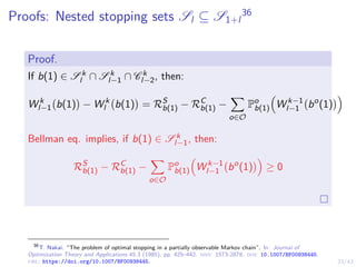
![20/43
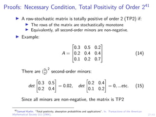
Proofs: S1 is convex18
b(1)
0 1
belief space B = [0, 1]
S1
α∗
1 β∗
1
18
Vikram Krishnamurthy. Partially Observed Markov Decision Processes: From Filtering to Controlled Sensing.
Cambridge University Press, 2016. doi: 10.1017/CBO9781316471104.](https://image.slidesharecdn.com/nyuinvitedtalkoptimalstoppinghammar30jan-230130171136-e7c97858/85/Intrusion-Response-through-Optimal-Stopping-71-320.jpg)
![21/43
Proofs: Single-threshold policy is optimal if L = 119
I In our case, B = [0, 1]. We know S1 is a convex subset of B.
I Consequence, S1 = [α∗, β∗]. We show that β∗ = 1.
I If b(1) = 1, using our definition of the reward function, the
Bellman equation states:
π∗
(1) ∈ arg max
{S,C}
150 + V ∗
(∅)
| {z }
a=S
, −90 +
X
o∈O
Z(o, 1, C)V ∗
bo
C (1)
| {z }
a=C
#
= arg max
{S,C}
150
|{z}
a=S
, −90 + V ∗
(1)
| {z }
a=C
#
= S i.e π∗
(1) =Stop
I Hence 1 ∈ S1. It follows that S1 = [α∗, 1] and:
π∗
b(1)
=
(
S if b(1) ≥ α∗
C otherwise
19
Kim Hammar and Rolf Stadler. “Learning Intrusion Prevention Policies through Optimal Stopping”. In:
International Conference on Network and Service Management (CNSM 2021).
http://dl.ifip.org/db/conf/cnsm/cnsm2021/1570732932.pdf. Izmir, Turkey, 2021.](https://image.slidesharecdn.com/nyuinvitedtalkoptimalstoppinghammar30jan-230130171136-e7c97858/85/Intrusion-Response-through-Optimal-Stopping-72-320.jpg)
![21/43
Proofs: Single-threshold policy is optimal if L = 120
I In our case, B = [0, 1]. We know S1 is a convex subset of B.
I Consequence, S1 = [α∗, β∗]. We show that β∗ = 1.
I If b(1) = 1, using our definition of the reward function, the
Bellman equation states:
π∗
(1) ∈ arg max
{S,C}
150 + V ∗
(∅)
| {z }
a=S
, −90 +
X
o∈O
Z(o, 1, C)V ∗
bo
C (1)
| {z }
a=C
#
= arg max
{S,C}
150
|{z}
a=S
, −90 + V ∗
(1)
| {z }
a=C
#
= S i.e π∗
(1) =Stop
I Hence 1 ∈ S1. It follows that S1 = [α∗, 1] and:
π∗
b(1)
=
(
S if b(1) ≥ α∗
C otherwise
20
Kim Hammar and Rolf Stadler. “Learning Intrusion Prevention Policies through Optimal Stopping”. In:
International Conference on Network and Service Management (CNSM 2021).
http://dl.ifip.org/db/conf/cnsm/cnsm2021/1570732932.pdf. Izmir, Turkey, 2021.](https://image.slidesharecdn.com/nyuinvitedtalkoptimalstoppinghammar30jan-230130171136-e7c97858/85/Intrusion-Response-through-Optimal-Stopping-73-320.jpg)
![21/43
Proofs: Single-threshold policy is optimal if L = 121
I In our case, B = [0, 1]. We know S1 is a convex subset of B.
I Consequence, S1 = [α∗, β∗]. We show that β∗ = 1.
I If b(1) = 1, using our definition of the reward function, the
Bellman equation states:
π∗
(1) ∈ arg max
{S,C}
150 + V ∗
(∅)
| {z }
a=S
, −90 +
X
o∈O
Z(o, 1, C)V ∗
bo
C (1)
| {z }
a=C
#
= arg max
{S,C}
150
|{z}
a=S
, −90 + V ∗
(1)
| {z }
a=C
#
= S i.e π∗
(1) =Stop
I Hence 1 ∈ S1. It follows that S1 = [α∗, 1] and:
π∗
b(1)
=
(
S if b(1) ≥ α∗
C otherwise
21
Kim Hammar and Rolf Stadler. “Learning Intrusion Prevention Policies through Optimal Stopping”. In:
International Conference on Network and Service Management (CNSM 2021).
http://dl.ifip.org/db/conf/cnsm/cnsm2021/1570732932.pdf. Izmir, Turkey, 2021.](https://image.slidesharecdn.com/nyuinvitedtalkoptimalstoppinghammar30jan-230130171136-e7c97858/85/Intrusion-Response-through-Optimal-Stopping-74-320.jpg)
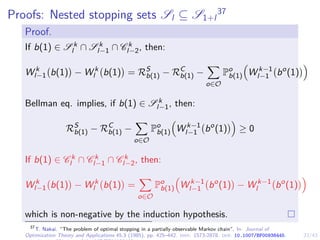
![22/43
Proofs: Single-threshold policy is optimal if L = 1
b(1)
0 1
belief space B = [0, 1]
S1
α∗
1](https://image.slidesharecdn.com/nyuinvitedtalkoptimalstoppinghammar30jan-230130171136-e7c97858/85/Intrusion-Response-through-Optimal-Stopping-75-320.jpg)
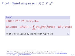
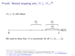
![31/43
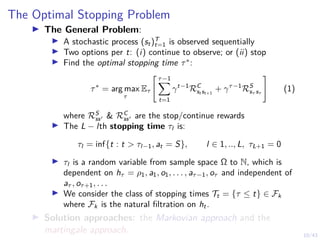
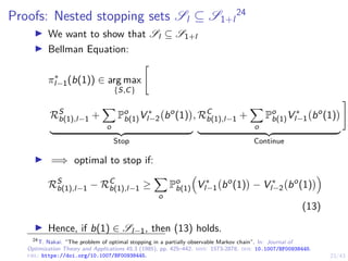
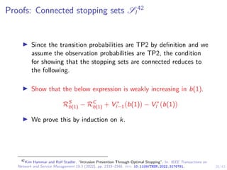
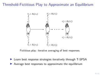
Proofs: Optimal multi-threshold policy π∗
l
49
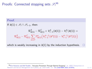
We have shown that:
I S1 = [α∗
1, 1]
I Sl ⊆ Sl+1
I Sl is connected (convex) for l = 1, . . . , L
It follows that, Sl = [α∗
l , 1] and α∗
1 ≥ α∗
2 ≥ . . . ≥ α∗
L.
b(1)
0 1
belief space B = [0, 1]
S1
S2
.
.
.
SL
α∗
1
α∗
2
α∗
L
. . .
49
Kim Hammar and Rolf Stadler. “Intrusion Prevention Through Optimal Stopping”. In: IEEE Transactions on
Network and Service Management 19.3 (2022), pp. 2333–2348. doi: 10.1109/TNSM.2022.3176781.](https://image.slidesharecdn.com/nyuinvitedtalkoptimalstoppinghammar30jan-230130171136-e7c97858/85/Intrusion-Response-through-Optimal-Stopping-103-320.jpg)
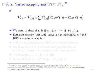
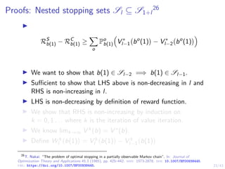
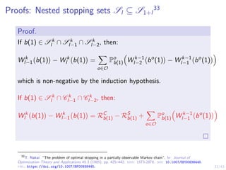
![32/43
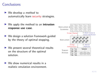
Structural Result: Best Response Multi-Threshold Attacker
Strategy
Theorem
Given the intrusion MDP, the following holds:
1. Given a defender strategy π1 ∈ Π1 where π1(S|b(1)) is
non-decreasing in b(1) and π1(S|1) = 1, then there exist
values β̃0,1, β̃1,1, . . ., β̃0,L, β̃1,L ∈ [0, 1] and a best response
strategy π̃2 ∈ B2(π1) for the attacker that satisfies
π̃2,l (0, b(1)) = C ⇐⇒ π1,l (S|b(1)) ≥ β̃0,l (16)
π̃2,l (1, b(1)) = S ⇐⇒ π1,l (S|b(1)) ≥ β̃1,l (17)
for l ∈ {1, . . . , L}.
Proof.
Follows the same idea as the proof for the defender case.
See50.
50
Kim Hammar and Rolf Stadler. Learning Near-Optimal Intrusion Responses Against Dynamic Attackers. 2023.](https://image.slidesharecdn.com/nyuinvitedtalkoptimalstoppinghammar30jan-230130171136-e7c97858/85/Intrusion-Response-through-Optimal-Stopping-104-320.jpg)

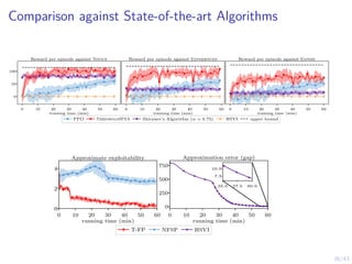


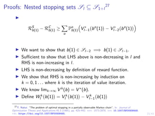
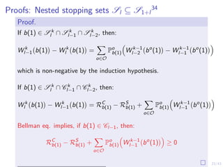
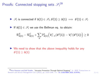
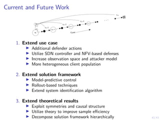
![41/43
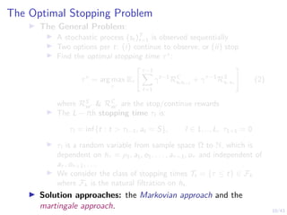
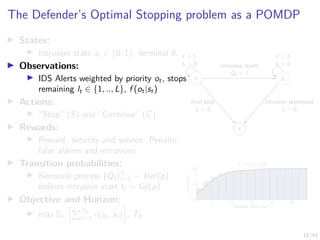
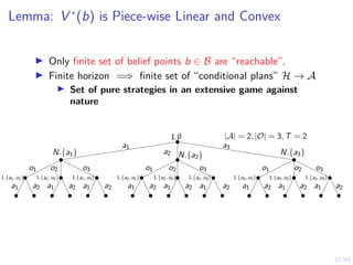
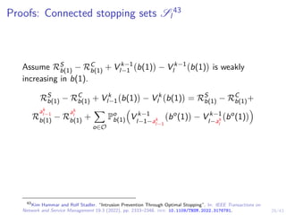
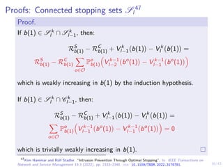
Learning Curves in Simulation and Digital Twin
0
50
100
Novice
Reward per episode
0
50
100
Episode length (steps)
0.0
0.5
1.0
P[intrusion interrupted]
0.0
0.5
1.0
1.5
P[early stopping]
5
10
Duration of intrusion
−50
0
50
100
experienced
0
50
100
150
0.0
0.5
1.0
0.0
0.5
1.0
1.5
0
5
10
0 20 40 60
training time (min)
−50
0
50
100
expert
0 20 40 60
training time (min)
0
50
100
150
0 20 40 60
training time (min)
0.0
0.5
1.0
0 20 40 60
training time (min)
0.0
0.5
1.0
1.5
2.0
0 20 40 60
training time (min)
0
5
10
15
20
πθ,l simulation πθ,l emulation (∆x + ∆y) ≥ 1 baseline Snort IPS upper bound](https://image.slidesharecdn.com/nyuinvitedtalkoptimalstoppinghammar30jan-230130171136-e7c97858/85/Intrusion-Response-through-Optimal-Stopping-120-320.jpg)

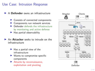
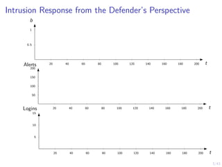
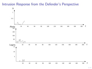
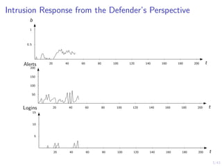
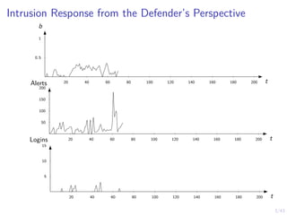
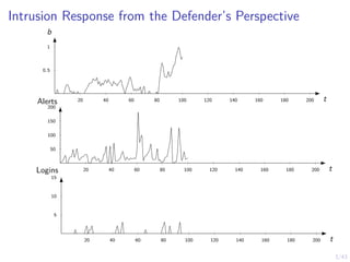
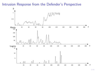
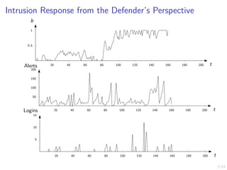
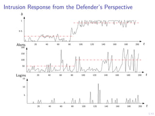
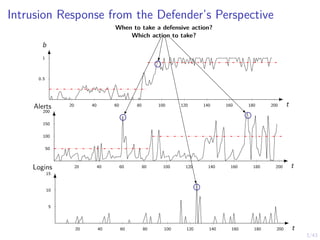
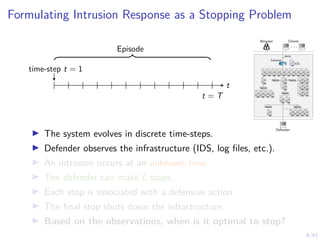
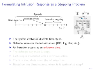
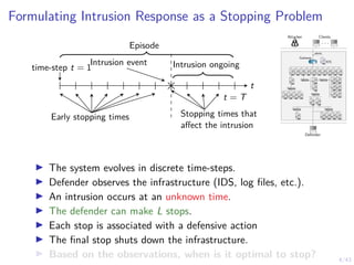
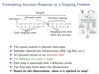
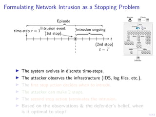
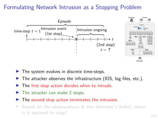
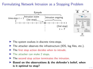
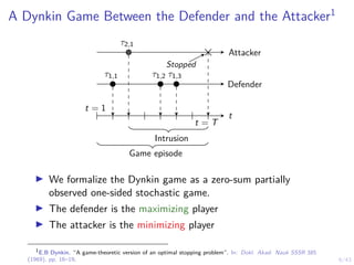
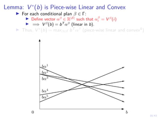
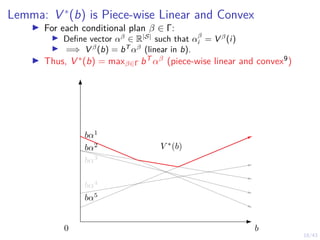
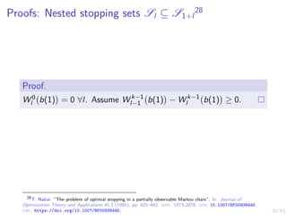
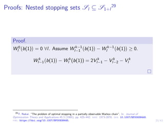
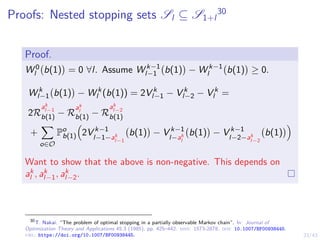
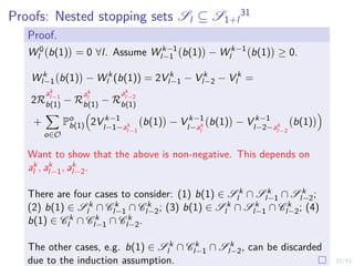
This document discusses formulating intrusion response as an optimal stopping problem known as a Dynkin game. The system evolves in discrete time steps with an attacker and defender. The defender observes the infrastructure and aims to determine the optimal time to stop and take defensive action based on observations. The approach involves modeling the interaction as a zero-sum partially observed stochastic game and using reinforcement learning to determine optimal strategies for both players.