J.B.Hunt_Inventory_Management_Report

1
Department of Industrial Engineering
4207 Bell Engineering
University of Arkansas
Fayetteville, Arkansas 72701
April 25, 2016
Reid Nelson, Operations Logistics Engineer
Jenni Kimpel, Director Engineering Services – Final Mile
J.B. Hunt Transport Services, Inc.
615 J.B. Hunt Corporate Dr.
Lowell, Arkansas 72745
Dear Mr. Reid Nelson and Ms. Jenni Kimpel:
Enclosed in this document is our team’s final project report. The report includes information
about J.B. Hunt and its services, specifically the Final Mile Segment. It also includes details
about the design of the project such as simulation results for over sixty Local Distribution
Centers and the parts that they carry.
The report details the objectives of the project, then describes our approach, tasks, and activities.
We then present the suggestions and results for each of the LDCs based on the data given from
the simulations. After presenting our recommendations the report breaks down the details of
working with both tools we used. The last section of the report is the appendix, which goes
through every step of the Arena Model and also includes details/instructions for the Visual Basic
program.
We hope this report gives an insight to the problem areas associated with the inventory problem
that are going on within the Final Mile Segment and its distribution centers. We would
appreciate your feedback on this report by Friday, April 29th. This feedback includes things such
as comments, corrections, or any other area you find needs changing. We know the report is
lengthy but this is due to the fact that we must analyze so many locations. We would also like to
thank you for working with us throughout the semester and being available to answer all of our
questions and concerns.
Respectfully,
Gavin Orgeron

2
University of Arkansas Industrial Engineering Design
J.B. Hunt Transport Services, Inc.
Final Mile Parts Inventory: Rough Draft
April 25th 2016
Submitted to:
Reid Nelson, Logistics Engineer
Jenni Kimpel, Director Engineering Services – Final Mile
Submitted by:
Team 4
Kevin Cobb
Dustin Jack
Gavin Orgeron, Project Manager
Travis Robbins

3
Executive Summary
Over the past year, most J.B. Hunt LDC managers order the max amount of parts they are
allowed to every order period. For most LDCs, this causes a huge amount of unnecessary
inventory to build up throughout the year. Using the program that we designed, we were able to
determine how much money could have been saved on ordering costs for J.B. Hunt. If every
manager ordered the max amount of parts every time they were allowed to order, J.B. Hunt
would have $10,144,500 of unused product sitting on their shelf. Although they get most of these
parts for free from Whirlpool, this is still causing massive pile-ups in inventory. These pile-ups
prevent the LDCs from running smoothly because they are unable to keep up with the entire
inventory they have on hand.
Once we realized that the inventories were building up to unnecessary amounts, we
decided to create rules to make it easier for the managers to determine how many parts need to
be ordered depending on what the current inventory is. We started by determining what the daily
demand was for each LDC. We then used this to determine how much safety stock each LDC
should keep on hand at any given time. We then wanted to create unique ordering rules for each
LDC to determine when they should order the max amount, a lower order quantity, or zero parts
depending on the current inventory.
The next step in our process was to create an Arena model to test our safety stock and
ordering rules for each LDC. We wanted to use the Arena model to determine how many times
they would have to go through a third party part supplier, NDA Distributors, to fill the demand.
Our goal was to minimize, if not eliminate, the need to use NDA. Using the Arena model, we
were able to test different rules to determine which values were the best to reduce the amount of
NDA orders while keeping the inventory at a manageable level. The hardest part about
implementing these rules is that each part in each LDC is unique depending on the yearly
demand.
In 2015 J.B. Hunt ordered 28,080 parts from NDA totaling a cost of $126,150. Using the
rules outlined in the report below, we were able to save J.B. Hunt over $50,718 in NDA ordering
costs. We only had to order 19,587 parts through NDA using the rules we came up with for each
individual LDC.
In order to implement our rules, the LDCs will be forced to come up with a way to track
the amount of inventory they have of each part. There is currently no way to track this, and this
is one of the reasons this problem has occurred. With a better organizational system in place, J.B.
Hunt should be able to save over $50,000.
Another obstacle we had to overcome was that we only had one year of data to work
with. This will limit our forecasting accuracy because of the short time period we were able to
look at. We recommend that as more data becomes available, J.B. Hunt should continue to revise
and edit the rules we have created. Once more data becomes available, the accuracy will increase
which will give J.B. Hunt a better idea of what the actual demand for each part in each LDC is.

4
Table of Contents
List of Tables .................................................................................................................................. 5
Project Overview........................................................................................................................... 10
1.1 Company Background Information .............................................................................. 10
1.2 Problem Information..................................................................................................... 11
1.3 Objectives...................................................................................................................... 13
1.4 Activities and Tasks...................................................................................................... 13
1.5 Conclusions, Recommendations, and Value to the Client............................................ 14
1.6 Future Research............................................................................................................. 16
Project Details............................................................................................................................... 17
2.1 Working with the Data.................................................................................................. 17
2.2 Creating the Models...................................................................................................... 19
2.2.1 Arena....................................................................................................................... 19
2.2.2 Visual Basic ............................................................................................................ 20
2.3 Analysis......................................................................................................................... 22
2.3.1 Atlanta Region........................................................................................................ 22
2.3.2 Carlisle Region....................................................................................................... 32
2.3.3 Columbus Region................................................................................................... 40
2.3.4 Dallas Region ......................................................................................................... 47
2.3.5 Denver Region........................................................................................................ 57
2.3.6 Orlando Region ...................................................................................................... 59
2.3.7 Perris Region.......................................................................................................... 63
2.3.8 Seattle Region......................................................................................................... 69
2.3.9 St. Louis Region..................................................................................................... 71
2.3.10 Chicago Region...................................................................................................... 75
2.4 Final Conclusions & Economic Analysis ..................................................................... 80
Appendix....................................................................................................................................... 83
Conclusion Tables......................................................................................................................... 83
VBA Program Instructions ........................................................................................................... 97
Explanation of the Arena Simulation Model ................................................................................ 99
References................................................................................................................................... 115

5
List of Tables
Table 1: Atlanta Simulation Results ............................................................................................. 22
Table 2: Atlanta Averages per Period........................................................................................... 23
Table 3: Birmingham Simulation Results..................................................................................... 23
Table 4: Birmingham Averages per Period .................................................................................. 24
Table 5: Dothan Simulation Results ............................................................................................. 24
Table 6: Dothan Averages per Period ........................................................................................... 24
Table 7: Knoxville Simulation Results ......................................................................................... 25
Table 8: Knoxville Averages per Period....................................................................................... 25
Table 9: Greer Simulation Results................................................................................................ 26
Table 10: Greer Averages per Period............................................................................................ 26
Table 11: Orangeburg Simulation Results.................................................................................... 26
Table 12: Orangeburg Averages per Period.................................................................................. 27
Table 13: Pensacola Simulation Results ....................................................................................... 27
Table 14: Pensacola Averages per Period..................................................................................... 28
Table 15: Chattanooga Simulation Results................................................................................... 28
Table 16: Chattanooga Averages per Period................................................................................. 28
Table 17: Garden City Simulation Results ................................................................................... 29
Table 18: Garden City Averages per Period ................................................................................. 29
Table 19: Charlotte Simulation Results ........................................................................................ 30
Table 20: Charlotte Averages per Period ...................................................................................... 30
Table 21: Raleigh Simulation Results........................................................................................... 30
Table 22: Raleigh Averages per Period ........................................................................................ 31
Table 23: Jacksonville Simulation Results ................................................................................... 31
Table 24: Jacksonville Averages per Period ................................................................................. 32
Table 25: Carlisle Simulation Results........................................................................................... 32
Table 26: Carlisle Averages per Period ........................................................................................ 33
Table 27: Norfolk Simulation Results .......................................................................................... 33
Table 28: Norfolk Averages per Period ........................................................................................ 34
Table 29: Richmond Simulation Results ...................................................................................... 34
Table 30: Richmond Averages per Period .................................................................................... 34
Table 31: Baltimore Simulation Results ....................................................................................... 35
Table 32: Baltimore Averages per Period..................................................................................... 35
Table 33: Chantilly Simulation Results ........................................................................................ 36
Table 34: Chantilly Averages per Period ...................................................................................... 36
Table 35: Boston Simulation Results............................................................................................ 37
Table 36: Boston Averages per Period ......................................................................................... 37
Table 37: Philadelphia Simulation Results ................................................................................... 37
Table 38: Philadelphia Averages per Period................................................................................. 38
Table 39: Edison Simulation Results............................................................................................ 38
Table 40: Edison Averages per Period.......................................................................................... 38
Table 41: Albany Simulation Results ........................................................................................... 39
Table 42: Albany Averages per Period ......................................................................................... 39

6
Table 43: Columbus Simulation Results....................................................................................... 40
Table 44: Columbus Averages per Period .................................................................................... 40
Table 45: Grayling Simulation Results......................................................................................... 41
Table 46: Grayling Averages per Period....................................................................................... 41
Table 47: Indianapolis Simulation Results ................................................................................... 41
Table 48: Indianapolis Averages per Period ................................................................................. 42
Table 49: Nashville Simulation Results........................................................................................ 42
Table 50: Nashville Averages per Period ..................................................................................... 43
Table 51: Clyde Simulation Results ............................................................................................. 43
Table 52: Clyde Averages per Period ........................................................................................... 43
Table 53: Louisville Simulation Results....................................................................................... 44
Table 54: Louisville Averages per Period..................................................................................... 44
Table 55: Cleveland Simulation Results....................................................................................... 45
Table 56: Cleveland Averages per Period..................................................................................... 45
Table 57: Detroit Simulation Results............................................................................................ 45
Table 58: Detroit Averages per Period ......................................................................................... 46
Table 59: Pittsburgh Simulation Results....................................................................................... 46
Table 60: Pittsburgh Averages per Period .................................................................................... 47
Table 61: Dallas Simulation Results............................................................................................. 47
Table 62: Dallas Averages per Period........................................................................................... 48
Table 63: Tulsa Simulation Results .............................................................................................. 48
Table 64: Tulsa Averages per Period ............................................................................................ 48
Table 65: Wichita Simulation Results .......................................................................................... 49
Table 66: Wichita Averages per Period ........................................................................................ 49
Table 67: Waco Simulation Results.............................................................................................. 50
Table 68: Waco Averages per Period ........................................................................................... 50
Table 69: Oklahoma City Simulation Results .............................................................................. 50
Table 70: Oklahoma City Averages per Period ............................................................................ 51
Table 71: Houston Simulation Results ......................................................................................... 51
Table 72: Houston Averages per Period ....................................................................................... 52
Table 73: Baton Rouge Simulation Results .................................................................................. 52
Table 74: Baton Rouge Averages per Period................................................................................ 53
Table 75: Shreveport Simulation Results ..................................................................................... 53
Table 76: Shreveport Averages per Period ................................................................................... 53
Table 77: San Antonio Simulation Results................................................................................... 54
Table 78: San Antonio Averages per Period................................................................................. 54
Table 79: Lubbock Simulation Results......................................................................................... 55
Table 80: Lubbock Averages per Period....................................................................................... 55
Table 81: Austin Simulation Results ............................................................................................ 56
Table 82: Austin Averages per Period .......................................................................................... 56
Table 83: McAllen Simulation Results......................................................................................... 56
Table 84: McAllen Averages per Period....................................................................................... 57
Table 85: Denver Simulation Results ........................................................................................... 58
Table 86: Denver Averages per Period ......................................................................................... 58
Table 87: Salt Lake Simulation Results........................................................................................ 58
Table 88: Salt Lake Averages per Period...................................................................................... 59

7
Table 89: Orlando Simulation Results.......................................................................................... 59
Table 90: Orlando Averages per Period........................................................................................ 60
Table 91: Tampa Simulation Results............................................................................................ 60
Table 92: Tampa Averages per Period.......................................................................................... 60
Table 93: Pompano Beach Simulation Results............................................................................. 61
Table 94: Pompano Beach Averages per Period........................................................................... 61
Table 95: Fort Myers Simulation Results ..................................................................................... 62
Table 96: Fort Myers Averages per Period ................................................................................... 62
Table 97: Perris Simulation Results.............................................................................................. 63
Table 98: Perris Averages per Period ........................................................................................... 63
Table 99: Santa Fe Springs Simulation Results............................................................................ 64
Table 100: Santa Fe Springs Averages per Period........................................................................ 64
Table 101: Las Vegas Simulation Results .................................................................................... 65
Table 102: Las Vegas Averages per Period .................................................................................. 65
Table 103: Hayward Simulation Results ...................................................................................... 65
Table 104: Hayward Averages per Period .................................................................................... 66
Table 105: Oxnard Remote Simulation Results............................................................................ 66
Table 106: Oxnard Remote Averages per Period ......................................................................... 66
Table 107: Phoenix Simulation Results........................................................................................ 67
Table 108: Phoenix Averages per Period...................................................................................... 67
Table 109: San Diego Simulation Results .................................................................................... 68
Table 110: San Diego Averages per Period .................................................................................. 68
Table 111: Fresno Remote Simulation Results............................................................................. 68
Table 112: Fresno Averages per Period ........................................................................................ 69
Table 113: Seattle Simulation Results .......................................................................................... 70
Table 114: Seattle Averages per Period ........................................................................................ 70
Table 115: Vancouver Simulation Results ................................................................................... 70
Table 116: Vancouver Averages per Period ................................................................................. 71
Table 117: St. Louis Simulation Results....................................................................................... 72
Table 118: St. Louis Averages per Period .................................................................................... 72
Table 119: Memphis Simulation Results...................................................................................... 72
Table 120: Memphis Averages per Period.................................................................................... 73
Table 121: Omaha Simulation Results ......................................................................................... 73
Table 122: Omaha Averages per Period ....................................................................................... 74
Table 123: Kansas City Simulation Results.................................................................................. 74
Table 124: Kansas City Averages per Period ............................................................................... 74
Table 125: Chicago Simulation Results........................................................................................ 75
Table 126: Chicago Averages per Period ..................................................................................... 75
Table 127: Des Moines Simulation Results.................................................................................. 76
Table 128: Des Moines Averages per Period ............................................................................... 76
Table 129: Milwaukee Simulation Results ................................................................................... 77
Table 130: Milwaukee Averages per Period................................................................................. 77
Table 131: Benton Harbor Simulation Results ............................................................................. 77
Table 132: Benton Harbor Averages per Period ........................................................................... 78
Table 133: Minneapolis Simulation Results ................................................................................. 78
Table 134: Minneapolis Averages per Period............................................................................... 79

8
Table 135: Davenport Simulation Results .................................................................................... 79
Table 136: Davenport Averages per Period .................................................................................. 79
Table 137: Simulation NDA Order Results .................................................................................. 81
Table 138: 2015 J.B. Hunt NDA Orders....................................................................................... 82
Table 139: Atlanta Rules & Suggestions ...................................................................................... 83
Table 140: Birmingham Rules & Suggestions.............................................................................. 83
Table 141: Dothan Rules & Suggestions ...................................................................................... 83
Table 142: Knoxville Rules & Suggestions.................................................................................. 83
Table 143: Greer Rules & Suggestions......................................................................................... 83
Table 144: Orangeburg Rules & Suggestions............................................................................... 84
Table 145: Pensacola Rules & Suggestions.................................................................................. 84
Table 146: Chattanooga Rules & Suggestions.............................................................................. 84
Table 147: Garden City Rules & Suggestions .............................................................................. 84
Table 148: Charlotte Rules & Suggestions................................................................................... 84
Table 149: Raleigh Rules & Suggestions ..................................................................................... 85
Table 150: Jacksonville Rules & Suggestions .............................................................................. 85
Table 151: Carlisle Rules & Suggestions ..................................................................................... 85
Table 152: Norfolk Rules & Suggestions ..................................................................................... 85
Table 153: Richmond Rules & Suggestions ................................................................................. 85
Table 154: Baltimore Rules & Suggestions.................................................................................. 86
Table 155: Chantilly Rules & Suggestions................................................................................... 86
Table 156: Boston Rules & Suggestions ...................................................................................... 86
Table 157: Philadelphia Rules & Suggestions.............................................................................. 86
Table 158: Edison Rules & Suggestions....................................................................................... 86
Table 159: Albany Rules & Suggestions ...................................................................................... 87
Table 160: Columbus Rules & Suggestions ................................................................................. 87
Table 161: Grayling Rules & Suggestions.................................................................................... 87
Table 162: Indianapolis Rules & Suggestions .............................................................................. 87
Table 163: Nashville Rules & Suggestions .................................................................................. 87
Table 164: Clyde Rules & Suggestions ........................................................................................ 88
Table 165: Louisville Rules & Suggestions.................................................................................. 88
Table 166: Cleveland Rules & Suggestions.................................................................................. 88
Table 167: Detroit Rules & Suggestions ...................................................................................... 88
Table 168: Pittsburgh Rules & Suggestions ................................................................................. 88
Table 169: Dallas Rules & Suggestions........................................................................................ 89
Table 170: Tulsa Rules & Suggestions......................................................................................... 89
Table 171: Wichita Rules & Suggestions ..................................................................................... 89
Table 172: Waco Rules & Suggestions ........................................................................................ 89
Table 173: Oklahoma City Rules & Suggestions ......................................................................... 89
Table 174: Houston Rules & Suggestions .................................................................................... 90
Table 175: Baton Rouge Rules & Suggestions............................................................................. 90
Table 176: Shreveport Rules & Suggestions ................................................................................ 90
Table 177: San Antonio Rules & Suggestions.............................................................................. 90
Table 178: Lubbock Rules & Suggestions.................................................................................... 90
Table 179: Austin Rules & Suggestions ....................................................................................... 91
Table 180: McAllen Rules & Suggestions.................................................................................... 91

9
Table 181: Denver Rules & Suggestions ...................................................................................... 91
Table 182: Salt Lake Rules & Suggestions................................................................................... 91
Table 183: Orlando Rules & Suggestions..................................................................................... 91
Table 184: Tampa Rules & Suggestions....................................................................................... 92
Table 185: Pompano Beach Rules & Suggestions........................................................................ 92
Table 186: Fort Myers Rules & Suggestions................................................................................ 92
Table 187: Perris Rules & Suggestions ........................................................................................ 92
Table 188: Santa Fe Springs Rules & Suggestions....................................................................... 92
Table 189: Las Vegas Rules & Suggestions ................................................................................. 93
Table 190: Hayward Rules & Suggestions ................................................................................... 93
Table 191: Oxnard Remote Rules & Suggestions ........................................................................ 93
Table 192: Phoenix Rules & Suggestions..................................................................................... 93
Table 193: San Diego Rules & Suggestions ................................................................................. 93
Table 194: Fresno Remote Rules & Suggestions ......................................................................... 94
Table 195: Seattle Rules & Suggestions....................................................................................... 94
Table 196: Vancouver Rules & Suggestions ................................................................................ 94
Table 197: St. Louis Rules & Suggestions ................................................................................... 94
Table 198: Memphis Rules & Suggestions................................................................................... 94
Table 199: Omaha Rules & Suggestions ...................................................................................... 95
Table 200: Kansas City Rules & Suggestions .............................................................................. 95
Table 201: Chicago Rules & Suggestions .................................................................................... 95
Table 202: Des Moines Rules & Suggestions............................................................................... 95
Table 203: Milwaukee Rules & Suggestions................................................................................ 95
Table 204: Benton Harbor Rules & Suggestions.......................................................................... 96
Table 205: Minneapolis Rules & Suggestions.............................................................................. 96
Table 206: Davenport Rules & Suggestions................................................................................. 96

10
Project Overview
1.1 Company Background Information
Johnnie Bryan Hunt founded J.B. Hunt, The Transportation Logistics Company, in 1961. The
company is based out of Lowell, Arkansas and primarily operates large semi-trailer trucks
throughout the continental United States, Canada and Mexico. J.B. Hunt started with five trucks
and seven refrigerated trailers to supply feed for chickens and by 1983 it had grown into the 80th
largest trucking firm earning $63 million in revenue. They are now employing over 16,000
employees and operate over 12,000 trucks; J.B. Hunt also owns over 47,000 trailers and
containers.
J.B. Hunt has a few different segments containing of: Dedicated Contract Service (DCS),
Intermodal (JBI), and Integrated Capacity Solutions (ICS). The DCS was started in 1992 and
“specializes in the design, development, and execution of supply chain solutions that support
virtually any transportation network.” [1] This division typically provides customized services
governed by long-term contracts. They operate dry-van, flatbed, temperature-controlled, dump
trailers and inner-city operations.
The Intermodal segment began operations in 1989 with a partnership with the BNSF
Railway Company. Currently, BNSF is used in the West and Norfolk Southern is used in the
East. Intermodal transportation uses different modes of transportation to move freight. So for
example, J.B. Hunt uses its own trucks but has a contract with BNSF to transport the container a
certain portion of the trip. This saves money for J.B. Hunt and creates business for the railway
companies. The Integrated Capacity Solutions include full truckload, dry-van freight using
company-controlled tractors operating over roads and highways. ICS also accounts for specialty
transportation services including Les-than-Truckload, refrigerated, and flatbed.

11
A smaller, less known service segment of J.B. Hunt is the Final Mile Segment (FMS).
The Final Mile is a network of cross dock distribution centers located in the lower contingent
United States and is considered to be a branch under the Dedicated Contract Service. There are
over eighty cross docks serving 98% of the population. Most of their business comes from
companies that are in need of solutions for their complex transportation issues. The FMS is
responsible for services including, but not limited to, drop-offs to appointment-generated white
glove deliveries. White glove service is a premium delivery service usually for larger items, such
as washers, dryers, and kitchen appliances. The service will generally deliver the item to the
destination and unpack, place, and install the appliance. After installation is complete, the
uniformed, capable, and well-trained J.B. Hunt employee will remove the packaging waste and
even remove the old appliance that is being replaced.
The FMS takes the pressures and responsibilities that are associated with deliveries away
from the partner that they do business with. This leaves the customer feeling safe and covered so
that they can focus on their core business.
1.2 Problem Information
The Final Mile Segment has experienced issues regarding the parts that are required for
installation of the appliances in which they deliver. Occasionally the inventory is out of stock
and cannot be used for installation; this delays the install and causes a second visit to a delivery
site. This is costing the FMS money and putting a damper on their reputation of having the
outstanding service for which they are so well known for.
The parts are items such as power cords for washer/dryers, hoses for refrigerator water line,
dryer vents, etc. They are ordered through the appliance company Whirlpool. Whirlpool and J.B.
Hunt have a contractual agreement that makes it easy for J.B. Hunt to order the parts that they

12
need. The Regional Distribution Center (RDC) or Local Distribution Center (LDC) will order
parts twice weekly, weekly, bi-weekly, monthly, or quarterly, depending on the volume of
demand they handle. As of now, FMS distribution centers will order the max amount from
Whirlpool for each SKU that they use. This results in large uncertainty in the amount of
inventory on hand and also makes for large amounts of unused parts that take up space in the
distribution centers. There are also occurrences of not having the part in inventory. When this
happens, J.B. Hunt must order through a third party company called NDA Distributors. These
parts are priced at a premium and cost both J.B. Hunt and Whirlpool a lot more money in the
long run.
Another issue within the FMS is the large order quantities associated with multi-family sites.
The multi-family service type is when there is an apartment building with many units, requiring
many appliances, thus, requiring many parts for these appliances. Not all of the LDCs cater to
the multi-family services but the ones who do must be prepared for when there is a large spike in
demand.
J.B. Hunt has asked our team to address their parts inventory problem by developing a model
that can help decide the demand of each RDC/LDC for each SKU and eliminate the need for the
3rd party vendor, NDA. The previous year’s data was given to us and we were granted the
freedom of choosing whichever method we saw fit for the problem at hand. This data includes
order numbers, order dates, what part(s) are ordered, quantity ordered, which LDC the order
came from, and the service type. This large file is the basis of our research and
recommendations.

13
1.3 Objectives
There are three objectives associated with the project description. The first was to document
current program’s objectives and how it is actually being executed. This is done by taking a look
at the order history and consulting with LDC managers on how decide on which parts to order.
The second objective was to create a forecast of orders for a year that require parts with
appliances. This objective was completed using a random number generator. When we took a
close look at the data we noticed that there weren’t any trends or seasonality. This led our group
to use the random number generator to create demand. We created these numbers based on the
mean and standard deviation of a normal distribution. The final objective was to outline new
options along with modeling how they should work. The problem description suggested that
simulation would be used to model the different policy options and how they interact with
delivery volume trends. Our group simulated future trends of each SKU in Arena Modeling
software for every LDC that met our requirements.
The project evolved over the course of the semester. We went from evaluating every LDC to
putting them into groups based on their demand. The smaller remote locations did not experience
enough demand to look at individually so we put them into a category that follows the same
guidelines throughout. For the larger LDCs, each location was evaluated differently.
1.4 Activities and Tasks
The areas that varied for each SKU: when the DC should order the max depending on the
amount of inventory, when they should order the recommended amount, safety stock, initial
inventory and the recommended order amount itself. The data file was used to find a normal
distribution for the demand of each part. This distribution was then implemented into the

14
simulation model to forecast the data for ten years. The main tasks of the project were analyzing
the data, creating a model for simulation, creating a program that focusses on the order periods
for specific parts/LDCs, and justifying our output in a way that proves our recommendations to
be economically viable.
1.5 Conclusions, Recommendations, and Value to the Client
Each LDC has its own unique recommendation. All of these individual recommendations can
be seen in the appendix. For our recommendation we will show what we think the initial
inventory and safety stock should be, what the distribution of orders was per day (mean, standard
deviation), how often multi-family orders came in (large orders are about 100), what the
inventory level is to decide if the max number of parts are needed, what the inventory level is to
decide if a different quantity should be ordered, what the NDA order quantity for that product is,
what the our max whirlpool order suggestion is, and how many parts should be ordered from
whirlpool if they are not ordering the max amount. There were some LDCs that didn’t have
enough demand throughout the year to justify a simulation, so our recommendation for those
sites is to maintain a safety stock that will allow them to meet their annual demand. For the small
LDCs, our group feels that a safety stock of ten of each part should allow these LDCs to fill their
demand without building up too much inventory.
The primary goal of the simulations we ran was to prevent the need for the LDCs to order
parts from a third party provider, NDA distributors. Our group understood that this would cause
an increase in inventory because we wanted to account for the variability that the LDCs
experienced throughout the year. We wanted to create certain rules that would easily allow the
LDC managers to keep track of when they need to order parts and how many they need. The
only problem is that there currently isn’t a way for the managers to keep track of how many parts

15
they have in the LDC. Our rules are based off the current number in inventory, so this will
require the managers to know exactly how many parts they have on site. An inventory
management system is needed in order to help the managers follow the rules we lay out.
The secondary goal of our simulation was to keep the lowest possible inventory on hand. Our
group understood that this goal was going to be more difficult to achieve because our main focus
was preventing the need for the 3rd party provider. We wanted to accomplish this goal by
creating situations where the managers don’t have to order the max amount of parts allowed
every single order period. Our rules are designed to allow the managers to order the max, none,
or a middle number of parts depending on how much inventory they have on hand. The number
of times the LDCs ordered these different quantities was a key statistic we kept track of in our
simulation model. If an LDC was able to order zero or a minimal amount of parts multiple times
throughout the year, we felt that we were helping decrease the overall inventory compared to
what it currently is.
There were multiple situations where we suggest that the LDCs should be allowed to raise
the max amount of parts allowed from whirlpool, and those situations are shown using red
numbers in those specific columns. The main reason we suggested that some LDCs should be
allowed to order more than the max amount of parts was the frequent occurrence of multi-family
orders. These multi-family orders forced the LDCs to keep a higher inventory on hand because
they have to be ready to fill these orders at any point throughout the year.
Once we were able to determine the appropriate safety stock for the LDCs, we would run
multiple simulations in order to determine what rules would best accomplish the two objectives
we talked about earlier. Although every LDC is unique we found a couple of patters in the rules
when we looked at all the recommendations. We would normally suggest that the LDC order the

16
max amount of parts allowed when their inventory was at half of the safety stock we initially set.
If the inventory was less than ¾ of the safety stock we would suggest that the LDC order less
than the max amount of parts allowed. Although each LDC is unique in the specific numbers,
this was the general layout of the rules we used when determining how many parts the LDC
should order at their given order period.
1.6 Future Research
The biggest issue regarding our project was the time period of the data. When we began the
project there was only order history for the year 2015. This hindered the ability to find trends.
Assumptions had to be made to account for the single year of data. It is assumed that the multi-
family orders occur in a manner that is considered constant and this is implemented in the
simulation model made for accompanying large multi-family orders.
In future research of the given problem, one may desire to implement a better organizational
policy for the LDCs and their inventory of parts. When our group visited the Tulsa LDC we
noticed that there was one storage rack where the parts were basically thrown into a pile with no
designation of where they should be placed. This will definitely account for a misrepresentation
of the inventory levels within the LDC. Tulsa is considered a smaller cross dock; this must be
considered when comparing the amount of inventory to hold and order per period. Without a new
inventory management system in place the LDCs won’t be able to implement the rules we put in
place because they won’t know their current inventory level is and how many parts are required.
This is critical for the success of the Final Mile program, because, not only will an inventory
management system help them figure out how many parts they need, but it will also make it
easier to locate parts and help the warehouses run smoother when they are getting parts ready for
orders.

17
Project Details
2.1 Working with the Data
We started by dividing all the data up by individual LDCs so that we could try to determine
what the demand would be throughout the year. We were able to use the order class to determine
what specific parts were going to be needed for each delivery. Once we were able to see when
specific parts were needed throughout the year, we wanted to try and create a forecasting model
to determine when parts needed to be ordered.
The first step in this process was to divide up the parts by the LDCs order period. This was
different for each LDC depending on whether or not they could order twice weekly, weekly, bi-
weekly, monthly, or quarterly. When we first did this we noticed that some of the larger LDCs
had huge spikes every couple of months where the demand for a certain part would sky rocket.
When we dove into the data we noticed that the majority of these were caused by large family
orders. When we talked to our sponsor he mentioned that these large family orders were
normally for installing appliances at the new apartments or complexes in certain cities. The
confusing part about these orders was that they could occur at any time without any warning.
The smaller LDCs would normally get a couple weeks’ notice to prepare for the order, but the
larger LDCs would have to make sure they had enough parts on hand to satisfy any family order
that came in throughout the year. The way we handled this problem was by trying to determine
how many family orders occurred on average throughout the year. We only had one year of data
to work with so we were uncertain as to whether or not the same pattern would occur in
following years.

18
Once we were able to separate the family orders from the normal deliveries we wanted to
forecast the demand for each part based on the order periods. We knew this was going to be
challenging to accurately forecast because there was only one years’ worth of data we could look
at. We originally tried to use moving averages to determine when parts would be needed but this
wasn’t very accurate for most of the LDCs because there was so much variance in the demand
for each order period. We then tried to determine if there was any seasonality we could use to
help predict when the most parts would be needed throughout the year. We logically thought that
the spring time would have a slight increase in orders because of tax refund season and the idea
that many people make large purchases at this time, but we couldn’t statistically prove that this
was true. We tried to use winter’s method to forecast with seasonality but the data didn’t have
enough correlation moving from one order period to the next. Dr. Chimka, the Industrial
Engineering department’s production planning and control professor, tried to help us look for
certain patterns in the data but we were unable to create a specific model that would work for all
LDCs.
The more we looked at the data we noticed that it just appeared to be random numbers. We
then used Minitab to create distributions of the order for each LDC. Most of the LDCs were able
to fit to a normal distribution. Minitab was able to give us the mean and standard deviation for
each part at each LDC, and we then used this information to create random number generators
that matched the demand for the parts. We felt that the random number generators was the best
way to forecast the demand because it was able to give a similar total number for the year, and it
would test our recommendations with the random spikes and decreases that occur throughout the
year. The random number generator was also a very easy way to implement our forecasting
predictions into the arena model we made.

19
2.2 Creating the Models
2.2.1 Arena
The focus of the Arena model was to estimate what the proper ordering quantity is for each
part for each LDC in order to minimize, if not eliminate, the need to order through the third
party, NDA Distribution. In order to achieve this multiple modules needed to be adjusted. The
first modules that were usually adjusted were the “Max Whirlpool Order” and “Receive
Whirlpool Order” ASSIGN modules. This is because if the LDCs are allowed to increase the
maximum order quantity than they will be receiving more parts from Whirlpool, which yields
more inventory on hand. With the extra inventory, the LDCs can fill more orders without
running out and having to order through NDA Distribution.
Along with adjusting these ASSIGN modules, it was also useful to adjust the “Inventory
Level to Decide” and the “Decide if Need Order” modules. By increasing the values in these
DECIDE modules, the number of NDA orders decreases. When the entity flows through the
“Inventory Level to Decide” module, the inventory is checked to see if it is below a certain level.
If it is then the maximum order quantity is placed. Since the specific inventory level is higher,
the LDC is forced to place more maximum orders than usual, which yield more parts on hand.
This again results in the LDCs being capable of filling more customer orders without running out
of inventory and minimizing the need to place an order through NDA Distribution. The purpose
of adjusting the “Decide if Need Order” module is similar to the reason for adjusting the
previous DECIDE module. This module checks if the current inventory is greater than, or equal
to, a much higher inventory level. If it is, then the LDC does not place an order to Whirlpool. If
it is less than the high inventory level the LDC will place an order to Whirlpool. Therefore, by
raising the inventory level in this module, it is more likely that the LDCs’ will be required to

20
place an order to Whirlpool for a smaller amount, rather than just not placing an order. Just as
before, this yields having more inventories minimizing the need to place an order through NDA
Distribution.
Another module that could be adjusted is the “NDA Order Filled” module. This is the
module that takes the amount from an NDA Distribution order and adds the amount to the
current inventory. Since the LDC is receiving more parts than normal they can again fill more
customer orders reducing the amount of times they have to order through NDA Distribution.
However, due to the price of NDA parts, this approach may be too expensive at times.
2.2.2 Visual Basic
After receiving the data it became clear that a sorting tool would be needed for quick
analysis. The potential of more data than the initial year given to us necessitated that this tool be
adaptable for multiple years. Initially the program focused on a ranking system by LDC but it
was quickly seen as unsupportive to the goals of our project. The final intended functionality
was decided after it became apparent that more data would be available and no demand
forecasting could be done. We approached Dr. Chimka for suggestions on how to deal with the
lack of diverse data and he suggested looking for gaps in the demand where the LDC would be
allowed to order more parts without actually needing them. This became the basis for the
program, as this could directly test if an LDC had an assigned order period that was appropriate
for its demand.
To accomplish this, data was to be sorted and made visual in such a way that a user could see
trends based on LDC and by ordering period. The value this program provided needed to be
focusing in on part cost for individual LDCs and the ordering process vs. actual demand.
Working on the assumption that an LDC will order the max allowed amount of parts and has

21
limited understanding of parts on hand we were able to create a model to compare actual demand
of parts to a year of ordering the maximum allowed parts per period. This was implied to be the
typical ordering procedure.
What the program provides the user is a comparison between the maximum an LDC is
allowed to order per period to what they needed throughout the year taken directly from the data.
There are two extremes on the spectrum, after visiting the Tulsa, OK LDC it became obvious
that some oversight was done on inventory levels but nothing near the careful tracking needed to
find and cut costs. So it would not be accurate to say that the LDCs blindly order parts when
they are swimming in them, however this description is not too far from the truth. It could be
assumed also that the cost calculated from demand would be the lower extreme or the optimal
cost if demand could be met perfectly.
This VBA program implemented to find a solution took the form of a pivot table that queried
the data and returned orders for the desired LDCs from a certain range of days based on the
departure date for the delivery. These orders were then sent through a table that matched the
order type to the parts required, multiplying these parts required by the number of appliances
ordered. Then these part counts were summed and printed in a new sheet. The other end of the
program was geared towards analysis, with premade “slates” that contained a table for the pivot
table to print into and graphical analysis of each part by order period. There is also a graph to
display the cost by part based on the produced table. The slates differ by ordering period and can
be updated as part costs change. The slate contains VBA code to move the results of the pivot
table into the next row of the slate. The slate then updates the graphs and total cost. When the
program is complete the results can be examined to see if the order period is a good fit by
comparing it to the policy that is or would be implemented.

22
When analyzing the data produced by the program, the user is looking for two scenarios for
every part. The first scenario is the LDC is ordering too often and there noticeable gaps in
demand for that part where it can be assumed that the LDC is ordering parts they do not have
demand for. The second scenario is the opposite; the LDC is using more parts than the max they
are allowed to order. Our analysis looked at the average parts ordered per period to compare to
what they were theoretically ordering. For the purposes of this analysis it was assumed that the
difference between the costs of ordering the max each period and the cost to fill actual demand
was the amount that JB Hunt could save by better fitting ordering policy to demand. However
since the pivot table can split the data in so many ways there are many uses for this program.
And with the ease at which it can adopt new data the data can be cut many different ways that
can then be put into the slates, which are not designed specifically for our analysis, but instead to
present the data the user wants to see.
Adding new data is as simple as copying and pasting the information into the sheet the pivot
table grabs the data from, extending and changing the selected data the pivot table uses.
2.3 Analysis
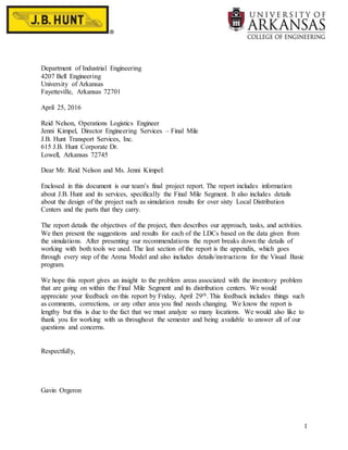
2.3.1 Atlanta Region
When we ran our simulation in the Atlanta region they had to order 2,435 parts, which
totaled to $11,410.22. We felt that our rules were successful in this region because of the size
of this region compared to some of the others.
Table 1: Atlanta Simulation Results
Atlanta (twice weekly) 4396020BULK 4396025BULK 8212638RP 20-3131-48A PT220L/400L/600L W10473735 30-3131-48 HOODPT3 PT220/400 4396897RW W10685193 8212560 4396672 4317824 3385556 8212486 W10505928RP
AVG Inventory 102 90 70 80 38 72 118 83 63 63 63 63 25 25 260
AVG Orders 10 10 9 10 5 5 20 7 3 3 3 3 3 3 26
Record 0 orders 49 41 36 33 30 61 11 53 64 64 64 64 5 5 12.2
Record MAX Orders 31 36 44 50 41 22 70 24 9 9 9 9 78 78 69
Record NDA Orders 8 9 10 9 10 8 12 8 1 1 1 1 7 7 1
Record Total Whirlpool Orders 90 89 89 89 88 91 88 90 90 90 90 90 88 88 90

23
After running our simulation, the Atlanta LDC required 93 NDA orders throughout the
year. This is not a bad percentage because we kept all of the max order quantities the same that
Whirlpool currently has them at. That is still only 6% of the total orders going through NDA.
Some of these orders can be associated with large variability in the demand and the random
family orders that comes in. We were able to keep the average inventory for every part at or
below the safety stock, which completes our secondary goal of minimizing the inventory.
Table 2: Atlanta Averages per Period
After analyzing the results of 2015 for L453 pulled from the data-sorting program, it was
found that the ordering policy currently used, twice weekly, is ineffective and should be
changed. Consider the table above. If the cell in the ‘Average per Period’ is highlighted in green
then it is demanded less than it is ordered to some degree and should be ordered less often. It is
suggested that this LDC considers the findings of our simulations for the safety stock kept and
amount ordered instead of using the current ordering policy. If demand is met solely by
Whirlpool this LDC has the potential to save $249,883.38.
Table 3: Birmingham Simulation Results
Birmingham required 23 NDA orders, which come out to 9% of the total orders for the
region. Although the NDA order where at a higher percentage for this LDC, we were able to
keep the inventory levels way below the safety stock.
20-3131-48A 30-3131-48 3385556 4317824 4396025BULK 4396672 4396897RW 8212486 8212560 8212638RP
Average per Period: 0.32 0.88 4.44 4.44 14.08 4.44 14.89 4.44 4.43 13.42
Max Allowed: 48 48 10 48 60 48 48 10 48 48
HOODPT3 PT220 PT220L PT400 PT400L PT600L W10505928RP W10685193 W10473735
Average per Period: 11.55 22.02 14.09 22.02 14.09 14.09 21.81 4.44 10.45
Max Allowed: 50 50 50 50 50 10 48 48 24
Birmingham (bi-weekly) 4396020BULK 4396025BULK 8212638RP 20-3131-48A PT220L/400L/600L W10473735 30-3131-48 HOODPT3 PT220/400 4396897RW W10685193 8212560 4396672 4317824 3385556 8212486 W10505928RP
AVG Inventory 89 84 77 79 14 21 75 21 122
AVG Orders 4 4 4 4 0 0 3 0 7
Record 0 orders 20 18 14 15 6 14 8 14 19
Record MAX Orders 0 0 0 0 0 1 5 1 0
Record NDA Orders 4 4 4 4 0 0 0 0 7
Record Total Whirlpool Orders 26 26 26 26 26 26 26 26 26

24
Table 4: Birmingham Averages per Period
found that the ordering policy currently used, biweekly, is ineffective and should be changed.
Consider the table above. If the cell in the ‘Average per Period’ is highlighted in green then it is
demanded less than it is ordered to some degree and should be ordered less often. It is suggested
that this LDC considers the findings of our simulations for the safety stock kept and amount
ordered instead of using the current ordering policy. If demand is met solely by Whirlpool this
LDC has the potential to save $86,745.97.
Table 5: Dothan Simulation Results
Dothan only required 2 NDA orders during our simulation. This is only 0.6% of the
orders coming through NDA, which we felt was a very successful result for our rules. Not only
were we able to almost completely eliminate the need for NDA, but also we were also able to
keep the inventory levels low compared to the safety stock.
Table 6: Dothan Averages per Period
20-3131-48A 30-3131-48 3385556 4317824 4396025BULK 4396672 4396897RW 8212486 8212560 8212638RP
Max Allowed: 48 48 10 48 60 48 48 10 48 48
Max Allowed: 50 50 50 50 50 10 48 48 24
Dothan (bi-weekly) 4396020BULK 4396025BULK 8212638RP 20-3131-48A PT220L/400L/600L W10473735 30-3131-48 HOODPT3 PT220/400 4396897RW W10685193 8212560 4396672 4317824 3385556 8212486 W10505928RP
AVG Inventory 25 24 24 24 15 28 24 40 33
AVG Orders 0 0 0 0 0 0 0 0 0
Record 0 orders 20 20 20 20 20 21 19 23 19
20-3131-48A 30-3131-48 3385556 4317824 4396025BULK 4396672 4396897RW 8212486 8212560 8212638RP
Max Allowed: 48 48 10 48 60 48 48 10 48 48
Max Allowed: 50 50 50 50 50 10 48 48 24

25
Table 7: Knoxville Simulation Results
Knoxville had 4 NDA orders during our simulation. This is only 1.3% of the total orders
going through NDA. All of the NDA orders were very similar parts with the same order
distribution. This can be attributed to the fact that Whirlpool only sells those parts in specific
packs rather than buying them individually.
Table 8: Knoxville Averages per Period
Knoxville (bi-weekly) 4396020BULK 4396025BULK 8212638RP 20-3131-48A PT220L/400L/600L W10473735 30-3131-48 HOODPT3 PT220/400 4396897RW W10685193 8212560 4396672 4317824 3385556 8212486 W10505928RP
AVG Inventory 41 36 27 36 29 31 31 32 32
AVG Orders 2 2 1 2 2 1 1 1 1
Record 0 orders 19 18 15 15 3 17 17 17 17
20-3131-48A 30-3131-48 3385556 4317824 4396025BULK 4396672 4396897RW 8212486 8212560 8212638RP
Max Allowed: 48 48 10 48 60 48 48 10 48 48
Max Allowed: 50 50 50 50 50 10 48 48 24

26
Table 9: Greer Simulation Results
Greer was an extremely successful LDC in testing our rules in the simulation. Our rules
were able to bring back no NDA orders for the LDC throughout the year. Not only were there no
NDA orders, but we were able to keep the average inventory relatively low throughout the year
as well.
Table 10: Greer Averages per Period
Table 11: Orangeburg Simulation Results
Orangeburg only required 1 NDA order during our simulation using the rules we
recommended. The one NDA order was for the amp range cords, and this can be attributed to the
Greer (bi-weekly) 4396020BULK 4396025BULK 8212638RP 20-3131-48A PT220L/400L/600L W10473735 30-3131-48 HOODPT3 PT220/400 4396897RW W10685193 8212560 4396672 4317824 3385556 8212486 W10505928RP
AVG Inventory 42 37 32 32 16 24 40 50 35 35 35 35 30 30 31
AVG Orders 1 1 1 1 1 1 2 1 0 0 0 0 0 0 1
Record 0 orders 20 19 17 17 12 18 13 17 20 20 20 20 1 1 17
20-3131-48A 30-3131-48 3385556 4317824 4396025BULK 4396672 4396897RW 8212486 8212560 8212638RP
Max Allowed: 48 48 10 48 60 48 48 10 48 48
Max Allowed: 50 50 50 50 50 10 48 48 24
Orangeburg (weekly) 4396020BULK 4396025BULK 8212638RP 20-3131-48A PT220L/400L/600L W10473735 30-3131-48 HOODPT3 PT220/400 4396897RW W10685193 8212560 4396672 4317824 3385556 8212486 W10505928RP
AVG Inventory 76 71 60 61 29 32 66 45 104
AVG Orders 3 3 3 3 2 2 6 2 7
Record 0 orders 36 33 26 30 26 28 16 37 4

27
high variability in demand for that product. Although we were required to order from NDA once
throughout the year, this was a successful simulation because we were able to prevent the
inventory from reaching too high of quantities.
Table 12: Orangeburg Averages per Period
found that the ordering policy currently used, weekly, is ineffective and should be changed.
Table 13: Pensacola Simulation Results
Pensacola required no NDA orders using our rules for the simulation. Not only did it not
require a single, but also they didn’t have to order the max quantity at all. This shows that our
rules allowed them to meet the demand without having to stockpile parts in the LDC. This
should help them with organization because they won’t have many parts that are not being used.
This allows them to cycle through inventory quicker without building up too high a number.
20-3131-48A 30-3131-48 3385556 4317824 4396025BULK 4396672 4396897RW 8212486 8212560 8212638RP
Max Allowed: 48 48 10 48 60 48 48 10 48 48
Max Allowed: 50 50 50 50 50 10 48 48 24
Pensacola (bi-weekly) 4396020BULK 4396025BULK 8212638RP 20-3131-48A PT220L/400L/600L W10473735 30-3131-48 HOODPT3 PT220/400 4396897RW W10685193 8212560 4396672 4317824 3385556 8212486 W10505928RP
AVG Inventory 25 23 23 23 23 21 23 21 21
AVG Orders 1 0 0 0 0 1 0 1 1
Record 0 orders 20 19 19 19 19 18 19 18 18

28
Table 14: Pensacola Averages per Period
Table 15: Chattanooga Simulation Results
Chattanooga required zero NDA orders during our simulation run. They also only
ordered the max a minimal amount of times for each part. This helped us keep the average
inventory at relatively low values compared to the safety stock that we originally recommended.
Table 16: Chattanooga Averages per Period
20-3131-48A 30-3131-48 3385556 4317824 4396025BULK 4396672 4396897RW 8212486 8212560 8212638RP
Max Allowed: 48 48 10 48 60 48 48 10 48 48
Max Allowed: 50 50 50 50 50 10 48 48 24
Chattanooga (bi-weekly) 4396020BULK 4396025BULK 8212638RP 20-3131-48A PT220L/400L/600L W10473735 30-3131-48 HOODPT3 PT220/400 4396897RW W10685193 8212560 4396672 4317824 3385556 8212486 W10505928RP
AVG Inventory 46 41 43 43 23 29 43 29 42
AVG Orders 2 2 2 2 1 1 2 1 2
Record 0 orders 19 17 12 12 9 9 12 9 13
20-3131-48A 30-3131-48 3385556 4317824 4396025BULK 4396672 4396897RW 8212486 8212560 8212638RP
Max Allowed: 48 48 10 48 60 48 48 10 48 48
Max Allowed: 50 50 50 50 50 10 48 48 24

29
Table 17: Garden City Simulation Results
Garden City only required one order from NDA during our simulation runs. This can be
attributed to the family orders that come in randomly throughout the year. If the manager is able
to know when a family order is coming and prepare for it then they should be able to prevent the
need for NDA at all.
Table 18: Garden City Averages per Period
Garden City (bi-weekly) 4396020BULK 4396025BULK 8212638RP 20-3131-48A PT220L/400L/600L W10473735 30-3131-48 HOODPT3 PT220/400 4396897RW W10685193 8212560 4396672 4317824 3385556 8212486 W10505928RP
AVG Inventory 22 19 20 31 17 38 60 26 112
AVG Orders 1 1 1 1 0 1 3 1 4
Record 0 orders 20 20 20 16 19 16 5 21 5
20-3131-48A 30-3131-48 3385556 4317824 4396025BULK 4396672 4396897RW 8212486 8212560 8212638RP
Max Allowed: 48 48 10 48 60 48 48 10 48 48
Max Allowed: 50 50 50 50 50 10 48 48 24

30
Table 19: Charlotte Simulation Results
Charlotte required no NDA orders when we used our rules. However, they were ordering
the max amount of parts about half the time throughout the year which shows that the current
max Whirlpool allows is a really good fit for this particular LDC. The rules that we have in place
seem to work for this LDC as well, and this can be seen in the row that shows how many times
the LDC orders zero parts. The inventory we set to prevent them from ordering any parts allows
them to maintain the right inventory while still being able to meet the demand for the parts.
Table 20: Charlotte Averages per Period
LDC has the potential to save $170644.99.
Table 21: Raleigh Simulation Results
Charlotte (weekly) 4396020BULK 4396025BULK 8212638RP 20-3131-48A PT220L/400L/600L W10473735 30-3131-48 HOODPT3 PT220/400 4396897RW W10685193 8212560 4396672 4317824 3385556 8212486 W10505928RP
AVG Inventory 81 79 66 75 37 56 74 55 87
AVG Orders 5 5 4 5 2 2 7 2 7
Record 0 orders 29 26 19 26 15 34 9 33 6
20-3131-48A 30-3131-48 3385556 4317824 4396025BULK 4396672 4396897RW 8212486 8212560 8212638RP
Max Allowed: 48 48 10 48 60 48 48 10 48 48
Max Allowed: 50 50 50 50 50 10 48 48 24
Raleigh (twice weekly) 4396020BULK 4396025BULK 8212638RP 20-3131-48A PT220L/400L/600L W10473735 30-3131-48 HOODPT3 PT220/400 4396897RW W10685193 8212560 4396672 4317824 3385556 8212486 W10505928RP
AVG Inventory 100 89 75 75 38 60 86 55 91
AVG Orders 4 5 4 4 2 2 6 2 5
Record 0 orders 67 65 60 60 60 76 56 73 59

31
Raleigh also had no NDA orders throughout the year. This LDC had one of the higher
demands for this region, and that can be seen in the fact they had a larger average inventory than
most of the other LDCs. Even with that being said, we were still able to keep the average
inventory at or below the recommended safety stock.
Table 22: Raleigh Averages per Period
After analyzing the results of 2015 for L856 pulled from the data sorting program, it was
found that the ordering policy currently used, Twice Weekly, is ineffective and should be
Table 23: Jacksonville Simulation Results
Jacksonville also did not require any NDA orders when we tested our rules in the simulation.
It shows that our rules are working when the table above shows that they didn’t have to order the
max amount of parts very often. This system of allowing them to choose how much they order
based on the current inventory helps prevent the average inventory from getting out of control.
20-3131-48A 30-3131-48 3385556 4317824 4396025BULK 4396672 4396897RW 8212486 8212560 8212638RP
Max Allowed: 48 48 10 48 60 48 48 10 48 48
Max Allowed: 50 50 50 50 50 10 48 48 24
Jacksonville (weekly) 4396020BULK 4396025BULK 8212638RP 20-3131-48A PT220L/400L/600L W10473735 30-3131-48 HOODPT3 PT220/400 4396897RW W10685193 8212560 4396672 4317824 3385556 8212486 W10505928RP
AVG Inventory 48 44 48 51 25 40 42 42 50
AVG Orders 2 2 2 1 1 1 1 1 3
Record 0 orders 35 32 35 36 34 42 42 42 30

32
Table 24: Jacksonville Averages per Period
2.3.2 Carlisle Region
Using our rules the Carlisle region was required to order 1,640 parts from NDA totaling
$7,353.15. We felt this was a good number to get because of the overall size of the region and
the number of LDCs we were dealing with.
Table 25: Carlisle Simulation Results
The Carlisle LDC only required seven NDA orders, which was 1.5% of the total orders
for the year. We felt this was a good result considering how often the program ended up ordering
the max number of parts. These NDA orders can be attributed to the variability in the demand
and the random spikes that occurred in one order period.
20-3131-48A 30-3131-48 3385556 4317824 4396025BULK 4396672 4396897RW 8212486 8212560 8212638RP
Max Allowed: 48 48 10 48 60 48 48 10 48 48
Max Allowed: 50 50 50 50 50 10 48 48 24
Carlisle (weekly) 4396020BULK 4396025BULK 8212638RP 20-3131-48A PT220L/400L/600L W10473735 30-3131-48 HOODPT3 PT220/400 4396897RW W10685193 8212560 4396672 4317824 3385556 8212486 W10505928RP
AVG Inventory 77 68 95 72 52 61 59 67 84
AVG Orders 4 4 3 4 3 3 3 3 3
Record 0 orders 31 23 41 31 29 31 32 32 38

33
Table 26: Carlisle Averages per Period
Consider the table above. If the cell in the ‘Average per Period’ is highlighted in red are
demanded more per period then they are allowed to order and these parts should be ordered more
to meet demand. However if this cell is highlighted green then it is demanded less than it is
ordered to some degree and should be ordered less often. It is suggested that this LDC considers
using the results of our simulations for the safety stock kept and amount ordered instead of using
the current ordering policy. If demand is met solely by Whirlpool this LDC has the potential to
save $87,584.78
Table 27: Norfolk Simulation Results
Norfolk also required 7 NDA orders, which were 3.2% of the total orders. Similar to
Carlisle, these NDA orders can be attributed to the variability that occurred during each order.
This can be seen in the number of max orders for each part. The small number of max orders
shows that there was probably a random spike in an order period, which caused the inventory to
drop to a very low level.
20-3131-48A 30-3131-48 3385556 4317824 4396025BULK 4396672 4396897RW 8212486 8212560 8212638RP
Max Allowed: 48 48 10 48 60 48 48 10 48 48
Max Allowed: 50 50 50 50 50 10 48 48 24
Norfolk (bi-weekly) 4396020BULK 4396025BULK 8212638RP 20-3131-48A PT220L/400L/600L W10473735 30-3131-48 HOODPT3 PT220/400 4396897RW W10685193 8212560 4396672 4317824 3385556 8212486 W10505928RP
AVG Inventory 69 49 45 45 38 43 43 46 58
AVG Orders 3 2 2 2 2 2 2 3 3
Record 0 orders 16 12 8 9 4 7 6 6 14

34
Table 28: Norfolk Averages per Period
Table 29: Richmond Simulation Results
Richmond only required three NDA orders using our rules. This comes out 0.6% of the
total orders going through NDA. Although we were able to prevent the need for the majority of
the NDA orders, the average inventory for the majority of the parts was a little high compared
the safety stock we originally set. This was one of the tradeoffs we had to make in order to
prevent the need for NDA.
Table 30: Richmond Averages per Period
20-3131-48A 30-3131-48 3385556 4317824 4396025BULK 4396672 4396897RW 8212486 8212560 8212638RP
Max Allowed: 48 48 10 48 60 48 48 10 48 48
Max Allowed: 50 50 50 50 50 10 48 48 24
Richmond (weekly) 4396020BULK 4396025BULK 8212638RP 20-3131-48A PT220L/400L/600L W10473735 30-3131-48 HOODPT3 PT220/400 4396897RW W10685193 8212560 4396672 4317824 3385556 8212486 W10505928RP
AVG Inventory 78 65 76 84 54 73 52 75 77
AVG Orders 2 2 2 2 2 2 2 2 2
Record 0 orders 40 37 40 39 21 36 32 37 37
20-3131-48A 30-3131-48 3385556 4317824 4396025BULK 4396672 4396897RW 8212486 8212560 8212638RP
Max Allowed: 48 48 10 48 60 48 48 10 48 48
Max Allowed: 50 50 50 50 50 10 48 48 24

35
Table 31: Baltimore Simulation Results
Baltimore didn’t require any NDA orders using our rules. Not only did they not require
any NDA orders, but also they rarely ever ordered the max amount of parts using the rules we
had in place. This was another case where we had to sacrifice the average inventory level in
order to prevent the need for NDA. The average inventory levels are only slightly above the
safety stocks we set for the parts.
Table 32: Baltimore Averages per Period
Baltimore (weekly) 4396020BULK 4396025BULK 8212638RP 20-3131-48A PT220L/400L/600L W10473735 30-3131-48 HOODPT3 PT220/400 4396897RW W10685193 8212560 4396672 4317824 3385556 8212486 W10505928RP
AVG Inventory 72 58 64 76 45 74 74 69 72 72 72 72 72 72 69
AVG Orders 2 2 2 2 2 3 3 3 2 2 2 2 2 2 3
Record 0 orders 33 31 34 35 16 33 33 30 33 33 33 33 33 33 31
20-3131-48A 30-3131-48 3385556 4317824 4396025BULK 4396672 4396897RW 8212486 8212560 8212638RP
Max Allowed: 48 48 10 48 60 48 48 10 48 48
Max Allowed: 50 50 50 50 50 10 48 48 24

36
Table 33: Chantilly Simulation Results
Chantilly required 13 total orders from NDA. This is only 0.7% of the total orders. It is
expected that this LDC would need NDA orders because of the large demand and variability. We
were still able to keep the average inventory at about the level of the safety stocks we had
originally set. We tried to find a middle ground between having too much inventory and needing
to order from NDA.
Table 34: Chantilly Averages per Period
After analyzing the results of 2015 for L728 pulled from the data sorting program, it was
found that the ordering policy currently used, Twice Weekly, is ineffective and should be
Chantilly (twice weekly) 4396020BULK 4396025BULK 8212638RP 20-3131-48A PT220L/400L/600L W10473735 30-3131-48 HOODPT3 PT220/400 4396897RW W10685193 8212560 4396672 4317824 3385556 8212486 W10505928RP
AVG Inventory 215 211 125 192 62 126 163 158 138 138 138 138 138 138 234
AVG Orders 16 15 11 16 4 5 12 11 8 8 8 8 8 8 17
Record 0 orders 64 56 39 53 47 75 63 58 62 62 62 62 62 62 61
20-3131-48A 30-3131-48 3385556 4317824 4396025BULK 4396672 4396897RW 8212486 8212560 8212638RP
Max Allowed: 48 48 10 48 60 48 48 10 48 48
Max Allowed: 50 50 50 50 50 10 48 48 24

37
Table 35: Boston Simulation Results
The Boston LDC required 8 NDA orders when we tested our rules in the simulation. This
was only 1.7% of the total orders for the year. Along with decreasing the need for the NDA
orders, we were also able to keep the average inventory at about the same level as our safety
stock. The large family orders that randomly come in would cause us to have huge inventories if
we wanted to completely eliminate the need for NDA.
Table 36: Boston Averages per Period
Table 37: Philadelphia Simulation Results
Boston (weekly) 4396020BULK 4396025BULK 8212638RP 20-3131-48A PT220L/400L/600L W10473735 30-3131-48 HOODPT3 PT220/400 4396897RW W10685193 8212560 4396672 4317824 3385556 8212486 W10505928RP
AVG Inventory 132 155 137 217 135 137 204 136 206
AVG Orders 16 17 17 17 4 3 14 3 16
Record 0 orders 1 1 2 18 12 12 20 12 0
20-3131-48A 30-3131-48 3385556 4317824 4396025BULK 4396672 4396897RW 8212486 8212560 8212638RP
Max Allowed: 48 48 10 48 60 48 48 10 48 48
Max Allowed: 50 50 50 50 50 10 48 48 24
Philadelphia (weekly) 4396020BULK 4396025BULK 8212638RP 20-3131-48A PT220L/400L/600L W10473735 30-3131-48 HOODPT3 PT220/400 4396897RW W10685193 8212560 4396672 4317824 3385556 8212486 W10505928RP
AVG Inventory 100 82 65 68 54 67 67 64 95
AVG Orders 4 4 4 4 3 4 4 4 8
Record 0 orders 34 24 21 22 8 20 20 18 4

38
Philadelphia only required two NDA orders during the year. This order can be attributed
to the large demand variability in the refrigerator hoses. The number of NDA orders would have
been much higher had we not suggested ordering more than the max that Whirlpool allows.
Table 38: Philadelphia Averages per Period
Table 39: Edison Simulation Results
Edison only required two NDA orders. The rules we had in place worked very well in
this LDC because there was a good mixture of ordering the max amount and a middle amount.
Table 40: Edison Averages per Period
20-3131-48A 30-3131-48 3385556 4317824 4396025BULK 4396672 4396897RW 8212486 8212560 8212638RP
Max Allowed: 48 48 10 48 60 48 48 10 48 48
Max Allowed: 50 50 50 50 50 10 48 48 24
Edison (weekly) 4396020BULK 4396025BULK 8212638RP 20-3131-48A PT220L/400L/600L W10473735 30-3131-48 HOODPT3 PT220/400 4396897RW W10685193 8212560 4396672 4317824 3385556 8212486 W10505928RP
AVG Inventory 97 80 64 66 45 68 66 63 63
AVG Orders 4 4 4 4 4 3 4 5 4
Record 0 orders 33 24 19 20 2 21 21 17 18
20-3131-48A 30-3131-48 3385556 4317824 4396025BULK 4396672 4396897RW 8212486 8212560 8212638RP
Max Allowed: 48 48 10 48 60 48 48 10 48 48
Max Allowed: 50 50 50 50 50 10 48 48 24

39
Table 41: Albany Simulation Results
Albany only required three NDA orders using the rules we had in place. Although we had to
order through NDA a couple of times, the average inventory level for each part was almost
exactly what we had planned for the safety stock which is a good sign that our rules are working
properly.
Table 42: Albany Averages per Period
Albany (bi-weekly) 4396020BULK 4396025BULK 8212638RP 20-3131-48A PT220L/400L/600L W10473735 30-3131-48 HOODPT3 PT220/400 4396897RW W10685193 8212560 4396672 4317824 3385556 8212486 W10505928RP
AVG Inventory 47 47 48 48 42 44 53 50 45
AVG Orders 2 2 2 2 2 3 2 2 2
Record 0 orders 10 0 11 11 0 10 12 11 10
20-3131-48A 30-3131-48 3385556 4317824 4396025BULK 4396672 4396897RW 8212486 8212560 8212638RP
Max Allowed: 48 48 10 48 60 48 48 10 48 48
Max Allowed: 50 50 50 50 50 10 48 48 24

J.B.Hunt_Inventory_Management_Report

J.B.Hunt_Inventory_Management_Report

Recommended

Recommended

More Related Content

Viewers also liked

Viewers also liked (6)

Similar to J.B.Hunt_Inventory_Management_Report

Similar to J.B.Hunt_Inventory_Management_Report (20)

J.B.Hunt_Inventory_Management_Report