2. 2 Lee, Yu-Yang
(1) Matrix Operations:
AI models rely heavily on matrix operations, such as matrix multiplications, which are
computationally intensive. Accelerators are optimized to efficiently perform these operations.
(2) Parallel Processing:
AI accelerators leverage parallel processing to perform multiple computations simultaneously,
accelerating training speed.
(3) Memory Hierarchy:
AI accelerators feature specialized memory architectures, including high-bandwidth mem-
ory (HBM) or on-chip memory, to minimize data movement and maximize memory access
bandwidth.
1.2 Cache design in AI accelerator
Cache is a vital element in contemporary computer architectures, including AI accelerators, as it
plays a crucial role in enhancing performance by reducing memory access latency. It is a small,
high-speed memory located in close proximity to the processing units. In AI accelerators, cache is
usually implemented in two locations: within the processing element (PE) and as a buffer RAM
situated between the DDR (main memory) and the PE array.
When the AI accelerator needs to fetch data, it first checks if the data is present in the cache. If it
is, it is considered a cache hit, and the data is accessed directly from the cache, resulting in faster
access time. If the data is not present in the cache, it is considered a cache miss. The data brought
into the cache is organized in cache lines or blocks, which are typically larger than the unit of data
accessed by the PE array.
Because AI workloads often exhibit high temporal and spatial locality, caches can capture and
retain this data, making it readily available for subsequent accesses. This minimizes the need to
repeatedly fetch data from memory, resulting in improved performance.
Also, by reducing memory access latency, cache enables processing units within the AI accelerator
to stay busy and avoid idling while waiting for data. This improves overall utilization and maximizes
the potential throughput of the accelerator.
1.3 The design of AIonChip
Fig. 1. The top-level architecture of AIonChip accelerator
The AIonChip system comprises three main components: PE arrays, Cache, and a Master CPU.
Communication for request and data transmissions occurs through the Network-on-Chip (NOC),
which consists of two channels: the Request channel and the Data channel. The NOC’s routers
, Vol. 1, No. 1, Article . Publication date: June 2023.
3. Cache simulator 3
connect each PE to form a network, facilitating the propagation of requests and data to the desired
PE using a handshaking mechanism.
The Master CPU is connected to the router located in the upper right corner.
Notably, on the right side of the NOC, four routers connect with cache controllers to map request
addresses to specific cache banks. Each cache bank is a functional unit capable of simultaneous
operation and is connected to DDR to retrieve data in case of cache misses.
The Master CPU initiates the computation process by sending write requests and multiple data
packets to the PE arrays. The PE’s internal DMA (as shown in Fig. 2) is activated, known as the
Program DMA. The DMA sends read requests to the cache to load firmware or loadables before
enabling the PCU/PTU. The NOC determines which router (e.g., cache bank) the request should be
directed to based on the data packet definitions.
Once the PCU/PTU’s firmware and loadables are loaded into its private SRAM, the PCU/PTU boots
up and begins loading input tensors, weight tensors, and lookup tables of the graph from the cache.
After the data is prepared, the PE initiates the subgraph inference process. Upon completion of the
inference, the output tensors are sent to other PEs or DDR for further processing.
Fig. 2. Internal architecture of PE
1.4 The effect of cache address mapping
According to the content in 1.2 Cache design in AI accelerator, the performance of an AI
accelerator is influenced by the cache design. This is because the most critical resources in an
AI accelerator are time spent on data movement and calculations. To optimize data movement
performance, it is crucial to ensure that data is in the right place at the right time. This is where
the address mapping of the cache plays a significant role.
In the AIonChip system, there are 16 cache banks, with each set of four banks connected to the
rightmost routers of the NOC. Currently, the cache controllers cannot directly communicate with
each other. Consequently, when a data request is sent to a specific cache bank, it must be routed to
the correct router connected to that bank, rather than any of the rightmost routers. This emphasizes
the importance of address mapping.
Consider a scenario where a subgraph of an AI model requires data from all PEs to be stored
in the first four cache banks (e.g., cache bank 0-3) based on the address mapping method. If all
PEs simultaneously request data, the requests will bottleneck at the same router, resulting in
sequential handling of requests and causing most PEs to idle. This diminishes parallelism and leads
to a significant drop in performance. In this scenario, an ideal solution is to assign each PE its
own request address within each cache bank. This ensures equal data distribution, allowing each
rightmost router to handle a maximum of four requests simultaneously. Moreover, the data for
, Vol. 1, No. 1, Article . Publication date: June 2023.
4. 4 Lee, Yu-Yang
each PE will be contiguous, facilitating more efficient data fetching.
However, this mapping method may not be suitable for all subgraph conditions. Consider a scenario
where a subgraph requires PE arrays to compute tensors with continuous addresses simultaneously.
Applying the previously mentioned address mapping method would assign the address of this
continuous tensor data to only one cache bank. As a result, all PEs would stall at the same router
until each request is handled one by one by the same cache bank, similar to the previous problem.
In this scenario, an ideal solution is to map the address based on the index number of the cache line.
This distributes the data across different cache banks, reducing the likelihood of PEs waiting for
the same cache bank to respond to data requests. This mapping method allows for the distribution
of continuous addresses to different cache banks, enabling different PEs to collaborate on the same
task simultaneously.
Based on the above discussion, it is evident that research on the address mapping method is vital.
AI accelerators need to handle various types of AI models, resulting in diverse workloads and data
read/write traces. Therefore, developing mapping methods tailored to different workloads becomes
an important consideration that significantly impacts performance.
2 CACHE SIMULATOR DESIGN
To explore the relationship between traces and address mapping, I will develop a cache simulator
capable of emulating the workflow of real traces being input into a cache system. This simulated
cache system will resemble the cache design depicted in Fig. 1.
2.1 Goal of the simulator
The primary objective of building this cache simulator is to analyze the effectiveness of various
address mapping strategies in different workloads. To achieve this goal, the simulator needs to
gather pertinent statistics, such as the simulated cycle count, enabling us to observe the outcomes
accurately. Additionally, the simulator is designed to interface with the AIonChip simulator to access
real traces from AI model graphs. To facilitate this, the simulator must support data transmission
with the NOC to communicate through the router’s data channel. Furthermore, the simulator
should be configurable, allowing it to simulate different types of models and workloads.
2.2 Features of the design
Fig. 3. Internal architecture of Cache system
, Vol. 1, No. 1, Article . Publication date: June 2023.
5. Cache simulator 5
Each cache bank in the system is connected to a memory NIC (also known as a Cache Con-
troller) and DDR. In this report, I will focus on a demonstration of a cache system consisting of
four cache banks. Each cache bank is equipped with several components, namely a request queue,
an LRU (Least Recently Used) table, a cache table, and an MSHR (Miss Status Handling
Register) queue. The purpose of each component is as follows:
(1) Request Queue:
To handle read/write requests from the NOC (Network-on-Chip) when the cache bank is
stalled, the following scenarios may occur when:
(a) The cache is waiting for DDR data to return. (b) Multiple requests are flowing into the
same bank.
If the request queue in a bank is full, that particular bank will not accept any more requests.
However, other banks can continue to handle requests from the NIC (Network Interface
Controller).
If a request from the NIC is sent to a bank with a full request queue, the NIC request pipeline
needs to wait until that specific bank accepts the request. As a result, the other banks cannot
accept requests even if their request queues are not full.
(2) MSHR queue & MAF queue:
The concept of non-blocking caches revolves around the idea of minimizing cache stalls when
cache misses occur. To achieve this, a register or queue called the Miss Status Holding
Register (MSHR) is utilized. The MSHR serves to keep track of whether a DRAM load
request has been completed and if subsequent instructions with the same address can be
executed. The MSHR comprises the following data components:
Fig. 4. The design of MSHR within cache bank
(a) three data to record the DDR load request:
• Valid (If MSHR entry valid/exist)
• Block address
• Issued (If the load request has issued to DRAM)
(b) four data to record PE load/store instructions:
• Valid (If instruction data valid)
• Type (Store/Load)
• Block offset
• Destination (The requested PE)
, Vol. 1, No. 1, Article . Publication date: June 2023.
6. 6 Lee, Yu-Yang
The above four data to record PE load/store instructions can be stored within a single module
known as the Miss Address File (MAF). The MAF has the capability to store multiple
requests that manipulate the same cache line when the corresponding cache index is already
present in an MSHR queue. In other words, the request data is currently being requested
from the DDR (main memory).
Note that block offset is needed when request data size is smaller than cache line size, it
can help to get the desired data location in the cache line. (e.g, If cache line size is 32 Bytes,
and the data PE requested is 16 Bytes, then block offset is needed to get the right 16 Bytes data.)
The workflow of MSHR:
• Cache Hits (Which means MSHR is not used)
• Cache Misses
1. Check if the requested address is inside MSHR. (If MSHR entry already exists)
2. If MSHR entry already exists, store instruction data (valid, type, block offset, destina-
tion) in MAF entry.
If MAF queue is full, this request will be hold until this specific MSHR entry data is
returned.
3. Else, creates a new MSHR entry, and request for data from DRAM.
A MSHR entry will not be issued immediately after it is created, MSHR queue will
check entry logged order, and issued one request in order in one cycle.
4. If MSHR entry is full, stall cache request handling.
Request queue can accept requests as usual, but this request will be handle until MSHR
queue has an empty entry.
• When data is loaded from DRAM to Cache
1. Check the instructions waited in MSHR entry, pass data and deallocate the instruction
request in order.
One MAF request will be handled in one cycle, so MSHR entry may not be deallocated
immediately after DDR data is return.
2. When stored instructions are all executed, deallocate this MSHR entry.
Fig. 5. Design of MSHR combine with MAF
(3) LRU table:
The LRU table is utilized when the cache is configured as an n-ways set-associative structure.
It serves the purpose of implementing the LRU (Least Recently Used) policy, which is a
, Vol. 1, No. 1, Article . Publication date: June 2023.
7. Cache simulator 7
commonly employed cache replacement policy. The LRU policy determines which cache
entry should be evicted when a cache miss occurs and there is a need to create space for a
new entry.
The LRU table is updated in two scenarios: when there is a cache hit or when the requested
data is retrieved from DDR. Upon a cache hit, the LRU table is modified to reflect the most
recently used entry. Conversely, when a cache miss occurs and data is fetched from the DDR
memory, the LRU table is updated accordingly.
In a set-associative cache, each cache line consists of multiple ways (entries). When all the
ways in a cache line are occupied, the cache follows the LRU policy to determine which way
should be replaced. The LRU table is consulted to identify the least recently used way, which
is then replaced with the new data. This ensures that the cache retains the most relevant and
frequently accessed data, maximizing cache hit rates and overall performance.
To gather a wider range of statistics and provide a more comprehensive analysis, the cache simulator
offers configurable options for the following settings:
• Total Cache Size
• N-Ways Set-Associative
• Cache Bank Number
• Cache Line Size
• Request Queue Entry Number
• MSHR Entry Number
• MAF Entry Number
• Address Mapping Mode
• Miss Penalty Cycle
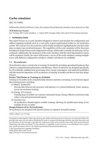
Another crucial aspect to specify is the Address Mapping Mode employed in the current cache
simulator design. Currently, there are only two available mapping methods, as depicted in Figure 6.
It is worth noting that Figure 6 is designed to demonstrate the mapping with 4 cache banks and 256
cache lines. The numbers shown in Figure 6 represent the cache line index numbers. In Mapping
Method 1, the cache line index for each bank is set to 64. On the other hand, Mapping Method 0
partitions the cache index into 4 portions.
0 4 8 12
.
.
.
.
.
240 244 248 252
Method 0
Method 1
1 5 9 13
.
.
.
.
.
241 245 249 253
2 6 10 14
.
.
.
.
.
242 246 250 254
3 7 11 15
.
.
.
.
.
243 247 251 255
0 1 2 3
.
.
.
.
.
60 61 62 63
0 1 2 3
.
.
.
.
.
60 61 62 63
0 1 2 3
.
.
.
.
.
60 61 62 63
0 1 2 3
.
.
.
.
.
60 61 62 63
Fig. 6. Address Mapping Method
• Mapping Method 0: This method assigns the request address to a cache bank based on
its cache line index number. In other words, requests with the same index will be di-
rected to the same cache bank. This method aims to evenly distribute consecutive address
, Vol. 1, No. 1, Article . Publication date: June 2023.
8. 8 Lee, Yu-Yang
requests among different banks. It performs well when the task at hand requires collaborative
computing from each processing element (PE).
• Mapping Method 1: This method assigns the request address to a cache bank based on its
most significant bit (MSB). In other words, requests with the same MSB in their addresses
will be directed to the same cache bank. The characteristic of this method is that it divides
the address space into N sections (N being the number of banks) and maps each section to
the corresponding bank based on its MSB.
2.3 Collaborative Integration of Cache System with NOC via IPC Channel in NOXIM
Fig. 7. Architecture of integration AIonChip simulator
The AIonChip simulator consists of four main components as shown in Fig. 7: the Cache
Simulator, the Master CPU, the NOC Simulator, and the IPC Memory Channel. The Cache
Simulator and Master CPU are implemented in C, while the NOC Simulator operates within NOXIM,
a simulation framework for Network-on-Chip (NOC) architectures based on System C. To facilitate
data transmission between the CPU, Cache, and NOC, the Linux IPC channel is utilized. This
channel offers a range of mechanisms and APIs for effective communication and synchronization
between processes.
It’s important to note that the system is currently in the development phase, and the integration of
these components is still a work in progress.
3 SURVEY OF TRACES
In this section, I will present a survey based on different traces with varying configurations. I
will analyze the trends observed in these traces, where only one configuration setting is changed.
Additionally, I will explain the validity of these trends based on the characteristics of the trace and
the altered setting. The purpose of this section is to demonstrate the impact of these factors and
establish the credibility of this cache simulator.
There are three traces, each showcasing a different type of locality, and the request of each trace is
to write.
• Loop: This trace consists of a big loop containing four distinct sequences of increasing
requests. Each sequence increments by 4 for a total of 500 iterations. The entire big loop is
repeated 600 times, resulting in a total of 1,200,000 input requests. This trace exhibits both
, Vol. 1, No. 1, Article . Publication date: June 2023.
9. Cache simulator 9
temporal locality and spatial locality due to the repetitive nature of the big loop and the
increasing patterns within each sequence.
• Forward: This trace consists of a single increasing request that increments by 4 for a total of
1,200,000 iterations. This pattern exhibits spatial locality as the requests are sequentially
accessed in memory.
• Random: This trace comprises 1000 randomly generated requests that are repeated for a
total of 1200 iterations. This pattern demonstrates temporal locality as the same set of
requests is accessed repeatedly within each iteration.
And below is the default configuration setting:
• Cache Size: 65536 Bytes (Fixed)
• N-Ways Set-Associative: 8
• Cache Bank Number: 4
• Cache Line Size: 32 Bytes (Fixed)
• Request Queue Entry Number: 4
• MSHR Entry Number: 8
• MAF Entry Number: 4
• Address Mapping Mode: 0/1
• Miss Penalty Cycle: 20 (Fixed)
3.1 N-Ways Set-Associative
Let’s first discuss the impacts of N-Ways Set-Associative changes:
(1) Cycles:
From Fig 8, we can see that only in the case of Random (Method 0), there is a noticeable
variation in Cycles. The characteristics of this trace involve 1000 random requests repeated
1200 times, and Method 0 evenly distributes consecutive memory locations across different
cache banks, so this mapping method does not have a significant impact on this trace. It can
be observed that Cycles are affected only when Ways are increased from Direct-Mapped
to 2-Ways Set-Associative. This can be attributed to the fact that duplicate Cache Indexes
will be replaced, and the initial increase in Ways becomes effective. Let’s compare Loop and
Forward: if Method 0 is used, it improves the efficiency by almost 2 times; for the Random
case, Method 1 performs better, but the difference between the two mapping methods is not
significant. This is because Loop and Forward both require processing a large contiguous
block of memory, and if Method 1 is used, the requests are concentrated in a few Cache Banks
for processing. Conversely, Method 0 can distribute this block of memory across different
Cache Banks to increase parallelism. In the case of Random, the reason for the minimal
impact of the two methods is that the request addresses are initially distributed randomly, so
the mapping method does not have a significant effect on performance.
(2) Hit Rate:
From Fig 8, we can see that increasing Ways results in a significant improvement in Hit rate
for all traces except Forward. Let’s analyze the Forward case from different perspectives. If we
judge solely based on the low Hit rate, we can conclude that the Forward trace does not reuse
the same Cache Line, and hence increasing Ways does not help. However, in the Forward
trace, the test data ranges from 0x0 to 0x493E00, involving 23 bits, so Cache Lines with the
same index will definitely be accessed repeatedly, and in considerable numbers. Therefore,
we can exclude this scenario. Another aspect to consider is the increase in miss rate due to
the Non-Blocking design. The inclusion of MSHR and MAF allows the Cache Bank to remain
functional even during misses, resulting in an increase in misses but a decrease in the number
, Vol. 1, No. 1, Article . Publication date: June 2023.
10. 10 Lee, Yu-Yang
Fig. 8. Trends of Changing Cache Ways (1)
Fig. 9. Trends of Changing Cache Ways (2)
Fig. 10. Trends of Changing Cache Ways (3)
of Cycles. By observing Fig. 9, we can find that in the Forward trace using Method 1, the
MSHR utilization is very low, but the MAF utilization is extremely high (close to 100%). This
is because all requests are stuffed into the same Bank, causing the later requests to need the
MSHR entries already issued in the previous requests, which are all pushed into MAF. As a
result, when using Method 1, the Hit rate approaches 0%. The situation is similar for Forward
using Method 0. Even though Method 0’s mapping allows all requests to be assigned to the
same bank, it still requires a large number of MAF entries. Additionally, Fig. 8 shows that
Method 0 can effectively reduce Cycles through MSHR design, but Method 1, due to poor
parallelism, increases Cycles even with heavy utilization of MAF.
, Vol. 1, No. 1, Article . Publication date: June 2023.
11. Cache simulator 11
(3) Writebacks:
From Fig 8, we can observe that writebacks decrease as Ways increase in the case of Loop
and Random traces. We can also see that the Hit rate for these two traces increases gradually
as Ways increase. This is because these traces have concentrated test data with repetition
at the same index, so increasing Ways effectively increases hits and reduces replacements,
resulting in a decrease in writebacks. However, for the Forward trace, the Hit rate does not
increase with Ways, so the number of writebacks does not decrease.
(4) Stall times:
MSHR Stall times calculate the number of times the cache bank stalls due to the MSHR queue
being full and unable to continue non-blocking operations. From Fig 10, it can be seen that
MSHR Stall times are affected to some extent as Ways increase in the case of Loop and Random
traces, especially when transitioning from Direct-Mapped to 2-Ways Set-Associative. This
is because Method 0 assigns cache banks based on the index, resulting in requests with the
same index being assigned to the same cache bank. This makes it easier for replacements to
occur when using Direct-Mapped. In the case of Random, because the addresses are randomly
generated, the occurrence of requests being assigned to the same cache bank due to Method
0 is less common compared to the Loop trace. In the Loop trace, most of the requests are for
contiguous memory, so they are always distributed to different cache banks by Method 0,
reducing the frequency of stall times. Therefore, increasing to 2-Ways Set-Associative can
alleviate this situation to a large extent. This can also be supported by the Hit rate shown in
Fig 8, where Random with Method 0 has a Hit rate of only around 60%.
3.2 Cache Bank Number
Let’s continue discussing the impacts of changing the Cache Bank Number:
(1) Cycles:
From Fig. 11, it can be observed that the cycles do not decrease with an increase in the bank
number for the Loop and Forward traces using Method 1. This is because in this mapping
method, only a single cache bank is assigned to requests, and even with an increased bank
number, it cannot be utilized for these two traces. On the other hand, traces using a better
address mapping method show a reduction in cycles with an increase in the bank number.
However, it can be seen that for the Loop and Forward traces, even with Method 0, there
is a significant decrease in cycles only when the bank number increases from 1 to 2. The
main reason for this is that a bank number of 2 or more is required for Method 0 to distribute
contiguous addresses to different banks. As for why there is no significant decrease in cycles
beyond a bank number of 2, it can be observed from Fig. 13 (Request queue stall times) that
as the cache bank number increases, the stall times in the request queue also increase. This
reduces the benefits of increasing the cache bank number to improve parallelism, resulting
in a similar number of cycles.
(2) Hit Rate:
From Fig. 11, it can be seen that except for the Loop trace using Method 1, the hit rate
increases to some extent with an increase in the cache bank number. The improvement is
particularly significant for the Forward trace using Method 0. This is mainly because with
an increased bank number and the assistance of the mapping method, contiguous memory
addresses are distributed to different cache banks, which not only helps with parallelism but
also improves the hit rate. With the same index being assigned to the same bank, cache lines
are more likely to be hit.
, Vol. 1, No. 1, Article . Publication date: June 2023.
12. 12 Lee, Yu-Yang
Fig. 11. Trends of Changing Cache Banks (1)
Fig. 12. Trends of Changing Cache Banks (2)
Fig. 13. Trends of Changing Cache Banks (3)
3.3 Request Queue Entry Number
Continue on discussing the impacts of changing the Request Queue Size:
(1) Cycles:
From Fig. 14, it can be seen that the cycles do not decrease with an increase in the request
queue size for the Loop and Forward traces using Method 1. The reasons for this have already
been discussed in the context of the bank number, so we will focus on discussing the trend for
the Loop and Forward traces using Method 0. When the request queue size increases, these
two traces show significant performance improvements. This indicates that within a short
period, there are more requests entering the same cache bank. This is mainly because these
two traces scatter contiguous memory addresses to different caches, causing consecutive
, Vol. 1, No. 1, Article . Publication date: June 2023.
13. Cache simulator 13
Fig. 14. Trends of Changing Request Queue Entry Number (1)
Fig. 15. Trends of Changing Request Queue Entry Number (2)
Fig. 16. Trends of Changing Request Queue Entry Number (3)
addresses of each cache line index to be read into the same cache bank, resulting in congestion.
This observation is also supported by Fig. 16 (Request queue stall times). Therefore, without
the temporary storage provided by the request queue buffer, traces with poorer mapping
strategies would require even more cycles. Thus, the size of the request queue has a significant
impact on cycles.
(2) Hit Rate:
From Fig. 14, it can be seen that the hit rate gradually decreases with an increase in the
request queue size for the Forward trace using Method 0. However, we can also observe from
Fig. 14 that the cycles are actually decreasing, and in some cases, they can even be lower
than those of the originally low hit rate Random trace. The reason for this is the effective
, Vol. 1, No. 1, Article . Publication date: June 2023.
14. 14 Lee, Yu-Yang
utilization of the non-blocking design. Method 0 scatters addresses evenly to different cache
banks, and with an increase in the request queue size, each cache bank has fewer chances of
experiencing congestion. At the same time, the MSHR (Miss Status Handling Register) and
MAF (Miss Address File) operate in sync. Therefore, even though the hit rate decreases, the
actual performance gradually improves.
3.4 MSHR Entry Number
Now we are discussing the impacts of changing the MSHR Entry Number:
Fig. 17. Trends of Changing MSHR Entry Number (1)
Fig. 18. Trends of Changing MSHR Entry Number (2)
Fig. 19. Trends of Changing MSHR Entry Number (3)
(1) Cycles:
From Fig. 17, it can be observed that the performance of the Forward trace is significantly
, Vol. 1, No. 1, Article . Publication date: June 2023.
15. Cache simulator 15
affected by the presence or absence of the MSHR (Miss Status Handling Register) design. This
is mainly because the Forward trace relies heavily on the MSHR and MAF (Miss Address File)
to hide the miss penalty. However, for all traces and both mapping methods, increasing the
MSHR Entry Number does not have a significant impact on cycles. This can be attributed to
the observation in Fig. 18, which shows that the utilization of the MSHR is not high in these
cases. Therefore, increasing the MSHR size does not improve performance significantly.
(2) Hit Rate:
The discussion regarding the decrease in hit rate has already been covered in the context of the
request queue size. However, the difference here is that for the Forward trace using Method
0, enabling the MSHR prevents further decrease in the hit rate. This reason is consistent with
the one discussed in the "Cycles" section. Since the utilization of the MSHR is not high in
these cases, increasing its size does not cause any significant impact.
3.5 MAF Entry Number
Lastly, we are discussing the impacts of changing the MAF Entry Number:
(1) Cycles:
Fig. 20 shows that in the case of the Forward trace, the MAF Entry Number has a greater
impact compared to the MSHR. This is because in the Forward trace, most requests are
contiguous, meaning they belong to the same cache line. Therefore, a larger MAF Entry
Number allows for more requests to be merged. However, the impact on other traces is not
significant. This can also be observed from Fig. 21, which shows that the utilization of the
MAF is higher only for the Forward trace, indicating that other traces do not require a large
number of same cache line writes (although this statement may have issues, as the Loop trace
theoretically also involves a large number of same cache line writes).
(2) Hit Rate:
Similarly, increasing the MAF Entry Number improves parallelism and enhances the per-
formance of the non-blocking design. As a result, the hit rate is reduced for the Forward
trace, but the actual performance is improved. For other traces, the impact of the MAF Entry
Number on hit rate is minimal, as explained in the "Cycles" section.
4 OBSERVATIONS AND TRENDS
Since the AIonChip simulator system has not been implemented yet, I have not had the opportunity
to observe real traces of workloads. As a result, I have not conducted an analysis on the relationship
between workloads and address mapping methods. This analysis will be performed once the entire
system is implemented.
5 SUMMARY
This report discusses a cache simulator designed to analyze and simulate the configuration and
address mapping methods used in a cache system within an AI accelerator. Where we introduce
the importance of AI accelerators in training AI models, emphasizing factors such as memory
bandwidth, energy efficiency, and scalability. The role of cache in improving performance is
explained, particularly in AI accelerators. The report presents the design of the AIonChip system,
including its components and communication channels. We also explores the effect of cache address
mapping on the performance of AI accelerators and discusses different mapping methods based on
various subgraph conditions. The cache simulator’s design is then described, outlining its goal of
analyzing address mapping strategies and its features, such as cache banks, request queues, LRU
tables, MSHR queues, and MAF queues.
, Vol. 1, No. 1, Article . Publication date: June 2023.
16. 16 Lee, Yu-Yang
Fig. 20. Trends of Changing MAF Entry Number (1)
Fig. 21. Trends of Changing MAF Entry Number (2)
Fig. 22. Trends of Changing MAF Entry Number (3)
, Vol. 1, No. 1, Article . Publication date: June 2023.