1. Initiating Factors and Physics of Landslide Tsunamis
Joshua S. Franck
Tsunamis are commonly referred to as shallow water waves that result from
seismic slip along a fault. Potential energy originates from stress along the fault
surface and is translated into wave energy. The incompressibility of water allows for
a majority of the energy to be translated into the wave crest. Resulting waves have
long wavelengths, on the order of 100 km, and propagate at high phase velocities, on
the order of 100 km/hr but with small initial amplitudes, usually only 1-5 m. These
ocean waves propagate radially outward in large bodies of water of varying depth
towards the shoreline, which results in waves slowing along the ocean floor.
Following the phase speed formula for shallow body waves, those where
wavelength (λ)>> Depth (H);
vphase = (g*H)0.5.
As waves enter shallower water, vphase decreases and as a result crest-amplitude
increases, which forms the large destructive waveforms which hit coastal regions.
Alternatively, Tsunamis can also be triggered when similar energy conditions
are appropriate. Firstly, an appropriately sized
body of water must be available for the wave to
propagate, and form a large enough wave crest.
In specific cases tsunamis can be generated in
bodies such as Lakes, Straits, Bays or
Reservoirs. Second, there must be an event of large initial energy to generate the
Figure 1

2. wave. In many cases this can result from Landslides (subaerial and subaqueous),
Volcanic eruptions or even Meteor impacts (cosmogenic)(Levin-Mikhail 2009). The
extent of this paper is limited to tsunamis generated in alternative water bodies by
landslides.
In two specific cases of landslide Tsunamis (LSTs), there is a dependence on
the initial impulse from the falling mass,
Lituya bay 1958, and by the water displaced
slide mass volume, Vajont reservoir 1963.
Note that either of these cases is not
primarily dependent on these two
illustrated factors but for the sake of
simplicity both cases will be analyzed as examples for these conditions.
As previously stated, LSTs are initiated by high-energy events, in this case landslides
where generally the volume of the slide ranges from 1-100 Mm3 (Crosta-
Imposimato 2013). These masses will range in elevation from orders of 10-100 m
above the waterline (Crosta-Imposimato 2013) and have densities from 2-3 g/cm3,
within range for rocks along a given coastal or lake shoreline (Twiss-Moores 1992).
Upon release, the slide mass can reach velocities of up to 110 m/s (Crosta-
Imposimato 2013). For example, a volume of 10^6 m3 of density 2 g/cm3 with a
frontal velocity of 50 m/s would have;
T=0.5*m*v2=0.5*ϱslide*Volslide*v2=0.5(2000kg/m3)(107m3)(20m/s)2
T=4*1012 J
Figure 2

3. As mass accumulates by either deposition or uplift (Twiss-Moores 1992), the
slope on which it adheres steepens (δ) and puts more stress (μ) on the lithological
boundaries which held the mass in place. The addition of mass results in greater
instability along the slope. In most cases instability is not the only factor to slide
events. In many examples of LSTs, slides are initiated by nearby seismic events, not
local enough to cause the Tsunami first hand but enough to generate a subsequent
slide. The most important note is that generally as potential energy increases,
instability increases proportionally.
Other factors, which can affect the instability of a material, are saturation of
the mass, usually after heavy rains, undercutting of material from heavy water flow
or nearby construction projects.
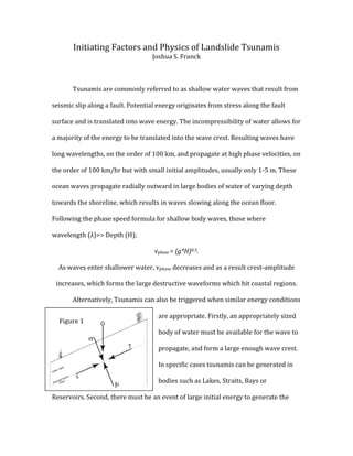
Slope failure can be most explained using the Safety Factor (SF) (Ritter
2004). SF is derived by first examining the force body diagram acting on the center
of mass of a body or slab of material, in this case consolidated slope material. Our
initial diagram (Figure 1) shows the normal stress of the material (σ), the
downward force on material acting on the slip surface, which is counteracted by the
pore pressure (μ). The materials position is maintained by the Shear strength of the
material (S), which is combination of forces opposing the shear stress (τ) that is
primarily composed of the cohesion of the material (C), and internal friction (at an
angle φ). Shear strength is given by the Coulomb equation;
Coulomb Equation: S=C+(σ-μ)tan(φ)

4. By representing the per/unit weight of the material as gamma and the height of
material as z, we can find the force of gravity (figure 2). From this we can define the
normal stress as;
σ=γ*z*cos(β)cos(β)
By adding additional material, in most cases water, but we can also assume
additional material (defined γw), we can represent the pore pressure;
μ=γ*m*z*cos(β)cos(β)
With m=Z/zw (zw=thickness added material). By this same notion shear stress is
represented by;
τ=γ*z*cos(β)sin(β)
With this notion, SF is then simply represented as the ratio of shear strength
over shear stress, SF=S/τ.
SF=S/τ=Shear Strength/Shear Stress
Where: 0<SF<∞
When SF=1, the slope is then determined to be balanced, but regarded as unsafe.
SF>1 is representative of stable slopes with larger values of SF correlating to more
stable conditions and. SF<1 is defined as slopes with instability. In cases where the
slope is unstable, is where slides occur.
Factors that could then reduce values of SF are γ*z=weight of overlying
material and the product of cos(β)sin(β), with beta being the angle of slip, with
cos(β)sin(β) increases to a maximum angle of β=π/4, where cos(β)=sin(β). This
makes sense as the angle of slide increases the value of Z will begin to approach
larger values, more simply, as β→π/2, z→∞. For the purpose of this paper we

5. assume SF≤1. The instance of SF=1 resulting in loss of stability is attributed to
seismic activity or other outside forces, leads to subsequent disturbances to
otherwise static material.
After losing stability the landmass moves as a super-viscous fluid along the
slope. The velocity field within the moving mass can then be interpreted as shearing
force acting along both the top and bottom of the moving material. We can then use
properties of moving viscous fluids (marked in notes) to estimate the velocity field
within the flow along the slope. Although the mass velocity gradient is interesting,
what is more important is the velocity of the flow front represented as an area h*z
with velocity vf. With this estimation we can then begin estimations as to the
strength of the impulse that initiates the Tsunami wave within the greater body.
One of the most notable values associated with the interactions between
slides and the resulting wave structures is the Froud number (F) (Fritz-Hager
2004). The Froud number is defined as;
F=vs/(g*D)0.5
Where: 0≤F≤∞
This value is also used in reference to the waves generated by a ship moving
through a liquid. Most notable in this function is the slide front to shallow water
phase velocity ratio, leading to relationship of F=1 corresponding to resonance
Figure 3

6. between the mass flow and the waveform. Simply put, if the slide is moving at the
same velocity of the resulting waveform, there is a significant increase in amplitude.
We will use the case of the Lituya landslide (1958) to illustrate the wave results
from an impulse, triggered from a nearby magnitude 7.7 earthquake 21 km away on
the Fairweather fault (Schwaiger-Higman 2007). The quake initiated the loss of 30
Mm3 from a mean elevation of 600 m above the water line which came rushing
down a 40° slope to an estimated max velocity of 110 m/s. The maximum thickness
of the slide was determined to be 92m, from comparing photographs before and
after the slide (figure 3), and the depth of the bay is considered to be 122m
(Schwaiger-Higman 2007). The first estimation that can be made is simply for the
Froud number for this interaction;
F=v/sqrt(g*D)=(110m/s)/(50m*10m/s2)0.5=4.9
From here we can already see that the situation is already close to resonance, within
a factor of 4, which partially explains such a large amplitude collision along the
adjacent shoreline (524m high!).
Through the use of a collision simulation between the waterline and the
viscous slide (Schwaiger-Higman 2007), it was determined that the resulting
waveform is more complex than a single radial wave. As is the case in many slides,
the overabundance of mass at high velocity induces turbulence, this is as expected if
we consider a high viscous flow interacting at low velocities. Examination of the
Reynolds number associated with the collision;
Re=L*v/η=(1Km)*(100m/s)/(1000kg/m3)=100

7. Where: 0≤Re<∞
From this we find solutions greater than 1 but still within
small values. Waves could be classified by their Froud
number (Fritz-Hager 2004) and separated into categories as
such;
F<(4-7.5S) where S=s/h nonlinear oscillatory (Note Figure4 with F vs. S)
(4-7.5S)≤F<(6.6-8S) nonlinear transition to Solitary waves
Froud numbers within these ranges are indicative of slides with high-energy slide
impact, resulting in oscillatory motion of fluid within the body. Froud values
representative of solitary waveforms vary within ranges of;
(6.6-8S)≤F<(8.2-8S) Solitary Waves
F≥(8.2-8S) Dissipative Bore
As far as the mechanics of the actual slide, they are discussed in Fritz’s paper
(Fritz-Hager 2004). The dimensions of the slide are estimated, from slide scarring,
with width and height 730 and 915m respectively and a maximum slide thickness of
92m, with a calculated volume of 30.6*106m3. Scale models depicting the slide event
(Figure 5, frames a-d) show the velocity vectors increasing around the shape of the
slide mass. Most notably in the first frames the velocity field is normal to mass the
front. Even in subsequent frames the velocity vectors from the first frames are still
oriented normal to the original slide geometry, even those where the fluid has lost
contact with the mass. In these cases the waveform is primarily influenced by the
front of the mass itself as it propagates through the fluid. In this case we refer back
to the previous mentioned potential energy and use it as a constraint for maximum
Figure 4

8. wave crest energy. Through the same modeling process (Fritz-Hager 2004), we can
estimate the loss of energy as the mass travels down slope. Using the kinetic energy
formula;
Es=0.5*ms*vs
2=4E12J
and using centroid velocity of the flow;
Vs=[2*g*Δz(1-f*cot(α)]0.5
Using this we can estimate the kinetic energy of the flow and compare to the original
potential, T=400 GJ;
U-T=600m*10m/s2*2000kg/m3-400GJ
ΔE=1.2E14J-4E11J=1.2E14J=0.997U
From this case we can see a loss of energy as the mass travels down-slope,
but only a small percentage. Here we have a representation of the multiple
regressions for the leading wave crest, as estimated in the Fritz paper which was
found experimentally and represented by the function;
Ac/h=0.25*(vs/sqrt(g*H))1.4*(s/h)0.8=0.25*F1.4*S0.8
Within the this value we can observe the relationship between the kinetic and wave
crest energy and their direct relation to the Froud number as well as the ratio of
slide thickness and collision depth and the slide volume over the product of slide
width to the square of the thickness. From the same experiment it was determined
that only 2-30% of the kinetic energy was transferred to the leading wave crest
(Fritz-Hager 2004).

9. The other extreme case would be that of the Vajont disaster of 1963. The
Vajont slide, similar to that of the Lituya event, displaced an area of 2 km^2 and an
estimated 275 Mm3 (Crosta-
Imposimato 2013). The mass
traveled down-slope at an angle of
17° to a maximum frontal velocity
of 20-30 m/s. The large volume
completely displaced the reservoir,
which at that point was about two
thirds full (115 Mm3 with an
average depth of H=100m). The
relative slide volume vs. reservoir
volume makes any sort of wave
structure, as previously illustrated
in the Lituya example, not viable. In
this case we neglect viscosity
altogether and treat the landslide
as a sliding block with an estimated
Froud number ranging between 0.26 and 0.75.
The result from the collision of the block into the reservoir sent water 140 m
up the opposing flank and 235m above the reservoir level and 100 m over the height
of the dam. The wave continued down the valley and towards the villages of
Figure 5

10. Longarone, Pirago, Rivalta, Villanova and Fae. The surge resulted in the deaths of
2000 people and transformed the valley into a muddy swamp.
Unlike the example of Lituya Bay, the slide did not result from an initial
seismic event, but by the loss of stability most likely due to lithologic boundaries
between stratigraphy, as seen in the geologic cross section in figure (Figure 6). This
difference would cause the cohesion to be much smaller than that of a homogenous
material. With loss of cohesion we can re-evaluate our Safety Factor for the slide.
Recall our safety factor represents the ratio of shear strength over shear stress. With
an already large amount of mass along the top of the boundary and a lowered
cohesion we can easily estimate a safety factor less than one. This example
illustrates the importance of evaluating civil engineering projects and possible
disasters that could result from their placement, relative to local geography.
After the collision the wave was estimated to undergo a series of oscillations
within the now altered reservoir
basin, raised significantly by the
slide. These oscillations are difficult
to understand as they did little to
erode the surrounding exposed
material, leaving scouring along the
shoreline. The subsequent wave had
significantly less amplitude then that
of the initial waveform, as a majority
of the water had already been displaced over the dam (Crosta-Imposimato 2013).
Figure 6

11. In both the cases of Lituya bay and the Vajont reservoir disaster slides where
most influenced by the high risen, steep slopes of material which had either a SF
value less then one or were triggered by an excess amount of energy, like that of the
Fairweather fault slip in Lituya bay. In most cases the volume of the slide is on the
same order of magnitude of that of the body of water it is interacting with, and in
some cases significantly greater. Slides that are significantly larger then the water
bodies they penetrate, like that of the Vajont disaster, are more importantly
characterized by the large volume of water displacement rather then resulting
waveforms. In these cases violent high-energy fluid is sent down geographic
gradients, which can lead to catastrophic results to any structures along the floods
path. In other cases the slide mass geometry most influences the waveform, taking
advantage of waters incompressibility. The mass displaces fluid normal to the slide
surface, accelerating the wave crest, transferring kinetic energy of the slide into
wave crest amplitude, shown in change of velocity vectors between frames through
experimentation (Schwaiger-Higman 2007).
With the primary factors for LSTs in mind, it is possible to assess high-risk
areas within California. Along the shoreline within most bays/inlets, there is high
damage potential especially that of the San Francisco bay area. Low depth values
within the bay present the potential for large Froud values which even further
represent a risk for Tsunami damage. Although the bay area is not at risk due to a
lack of high rising slopes above one hundred meters above the waterline or within
close enough proximity for high velocity mass to reach the water before energy is
dissipated due to friction along the slide pathway. Another high-risk region would

12. be the eastern banks of Lake Tahoe. The slopes reach up to 400 m above the
waterline with slopes leading directly into the lake. This creates the potential for
large volumes of high velocity material to make contact with the fluid and instigate a
waveform such as in Lituya bay. In this case though the surface area of the lake is
substantial and provides a large region for the wave to propagate. As seen in the
damage following the Lituya tsunami, the wave amplitude was largest when
powered by the motion of the landslide along the lake bottom. In this case the slide
would come to rest after some several hundred meters, allowing the wave to
dissipate radially throughout the lake surface.
One example that presents a significant danger is that of a possible event in
Trinity Lake, located 46 km Northwest of Redding Ca. The lake is a man-made
reservoir, which is one of the largest in California. The lake itself is composed of
several inlets that were previously gorges between nearby mountains. In some
cases the slopes rise up several hundred meters above the water column and lead
directly to the lake surface. Furthermore some of the steepest slopes which hold the
highest slide potential are those which are only one kilometer away from the man
made dam. The possibility of a waveform such as the one Lituya bay, overriding the
dam and traveling down towards Lewton Lake and Lewton itself, as happened in
Vajont, is very likely. Considering the seismic activity in California due to contact
between the North American and Pacific Plate, including that of the San Andreas
Fault, it is more likely that even slopes with SF>1 to be triggered by additional
energy from ground waves from large magnitude earthquakes.

13. Works Cited
Levin, Boris, and Mikhail Nosov. "Physics of Tsunami Formation by Sources of
Nonseismic Origin." Physics of Tsunamis. Dordrecht: Springer, 2009. Print.
Fritz, H. M., W. H. Hager, and H.-E. Minor. "Near Field Characteristics of Landslide
Generated Impulse Waves." Journal of Waterway, Port, Coastal, and Ocean
Engineering (2004): 287-300. ASCE Library. American Society of Civil Engineers.
Mon. 1 Dec. 2014. www.ascelibrary.or
Jiang, L., and P. H. Leblond. "The Coupling of A Submarine Slide and The Surface
Waves Which It Generates." Journal of Geophysical Research (1999): 12731-
2744. Wiley Online Library. John Wiley & Sons, Inc. Mon. 1 Dec. 2014.
www.onlinelibrary.wiley.com.
Crosta, Giovanni B.., Silvia Imposimato, and Dennis Roddeman. "Interaction of
Landslide Mass and Water Resulting in Impulse Waves." Landslide Science and
Practice5 (2013): 49-56. Springer Link. Springer International Publishing. Web. 28
Nov. 2014. www.link.springer.com.
Ritter, John B.. "Landslides and Slope Stability Analysis." Wittenberg University.
Wittenberg University, Springfield, OH. 1 Jan. 2004. Lecture.
Twiss, Robert J., and Eldridge M. Moores. Structural Geology. New York: W.H.
Freeman, 1992. Print.
Schwaiger, H. F., and B. Higman. "Lagrangian Hydrocode Simulations of the 1958
Lituya Bay Tsunamigenic Rockslide." Geochemistry Geophysics Geosystems 8.7
(2007). Wiley Online Library. John Wiley & Sons, Inc. Web. 5 Dec. 2014.
www.onlinelibrary.wiley.com.
Wiegel, R., & J. W. Johnson. "ELEMENTS OF WAVE THEORY." Coastal Engineering
Proceedings [Online], 1.1 (1950): 2. Web. 16 Dec. 2014