FLARE Final Report

FLyby Anomaly Research Endeavor
FLARE Final Report
Graeme Ramsey, Jeffrey Alfaro, Amritpreet Kang, Kyle Chaffin, and Anthony Huet
May 08, 2015
ASE 374L Spacecraft/Mission Design: Dr. Fowler
The University of Texas at Austin
In conjunction with JPL: Travis Imken and Damon Landau
Spring 2015
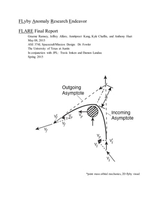
*point mass orbital mechanics, 2D flyby visual

Table of Contents
Executive Summary
1.0 Introduction
1.1 Heritage
1.1.1 Initial Observations
1.1.2 Heritage Missions
1.1.3 Phenomenological Formula
1.2 Mission Motivations
1.3 Unconfirmed Explanations of the Flyby Anomaly
1.3.1 Dark Matter Encircling the Earth
1.3.2 Modifications in Inertia
1.3.3 Special Relativity
1.3.4 Lorentz Accelerations
1.3.5 Anisotropy of the Speed of Light
1.3.6 Perturbing Force Error
1.3.7 Modeling Error
1.3.8 JUNO Findings: Higher Order Gravity Terms
1.4 Mission Constraints and Assumptions
1.5 Report Preview
2.0 Driving Statements and Requirements
2.1 Scope
2.1.1 Need
2.1.2 Goal
2.1.3 Objectives
2.1.4 Mission
2.1.5 System Constraints
2.1.6 Assumptions
2.1.7 Authority and Responsibility
2.2 Primary Requirements
2.2.1 Mission Requirements
2.2.2 System Requirements
2.2.3 Requirements Traceability Matrix
3.0 System DesignDevelopment
3.1 Design Alternatives Development
3.1.1 Preliminary ConOps 1

3.1.4 Primary ConOps
3.1.5 Secondary ConOps
3.2 Selection of ConOps
3.3 System and Subsystems Allocation
3.4 Design Heritage
3.4.1 INSPIRE CubeSat
3.4.2 X/X-band LMRST
3.4.3 Iris X-band Transponder
3.4.4 GPS/GNSS Receivers Overview
3.4.5 Satellite Laser Ranging
3.5 Trade Study Summary and Results
3.5.1 Data Acquisition Systems Capabilities
3.5.2 Launch Vehicle
3.5.3 Trajectory
3.5.4 Ground Station Tracking
3.5.5 Trajectory Separation
3.5.6 Propulsion
3.5.7 Prospective Modeling Analysis
3.6 Critical Parameters
4.0 System Design
4.1 Baseline Mission Designs
4.1.1 Primary ConOps A Baseline Trajectory
4.1.2 Secondary ConOps B Baseline Trajectory
4.1.3 Velocity Maneuver Budget
4.1.4 Post-Launch and Deployment Details
4.1.5 Day in the Life of FLARE
4.2 Satellite Design Choices
4.2.1 System and Subsystem Overview
4.2.2 Master Equipment List (MEL)
4.2.3 Equipment Volume Allocation List (EVAL)
4.2.4 Power Equipment List (PEL)
4.2.5 Comms Link Budget and EbNo Analysis
4.3 Mission Timeline and Schedule
4.4 Cost Analysis
4.5 Risk Analysis
4.6 Economics, Environmental and Sustainability Issues
4.7 Ethical, Social and Health/Safety Issues
4.8 Manufacturability, Political and Global Impact Issues

5.0 DesignCritique
5.1 Strengths
5.2 Weaknesses
5.3 Confidence
5.4 Alternatives
5.5 Remaining Design Refinements
5.5.1 CAD Model for Analysis
5.5.2 Trajectory Refinement
5.5.3 Comms Link Budget
6.0 Summary and Conclusions
7.0 References
7.1 Image References
8.0 Appendices
Appendix I: Primary Resources Reference Information
Appendix II: FLARE Team Management
Appendix III: Subsystem Requirements
Appendix IV: JPL Feedback

List of Tables
Table 1: Flyby orbital parameters of heritage missions
Table 2: Heritage missions navigation
Table 3: Primary requirements traceability matrix
Table 4: LMRST comms link budget
Table 5: Noise from various LEO benchmark tests
Table 6: Steady state GPS navigation errors
Table 7: Visibility and Slew Rate for potential tracking systems
Table 8: Thermal requirements
Table 9: Baseline trajectory data, ConOps A departure and heliocentric
Table 10: Baseline trajectory data, ConOps A flybys
Table 11: Baseline trajectory data, ConOps B flyby
Table 12: DeltaV Budget
Table 13: Design selection criteria
Table 14: MEL - Master Equipment List
Table 15: EVAL - Equipment Volume Evaluation List
Table 16: PEL - Power Equipment List - Nominal
Table 17: Power Production at 40% and 70% Output
Table 18: Orbital correction maneuver power
Table 19: Desaturation maneuver power
Table 20: Flyby power
Table 21: IRIS Comms Link Budget
Table 22: Component-wise cost estimation for one 6U cubesat
Table 23: Phase D through F cost estimation for two 6U CubeSats
Table 24: Risk Register for the Spacecraft
List of Figures
Figure 1: Magnitude of Potential Error Sources
Figure 2: Simulated Doppler residuals from 7 mm/s anomaly
Figure 3: JUNO Doppler postfit residuals reconstruction and deleted data
Figure 4: Position and velocity perturbations from higher order gravity terms
Figure 5: CSD dispenser deployment setups
Figure 6: Sherpa on payload section
Figure 7: Primary ConOps
Figure 8: Secondary ConOps
Figure 9: FLARE Primary ConOps PBS
Figure 10: INSPIRE cubesat
Figure 11: Downlink rates for INSPIRE using Iris
Figure 12: JPL LMRST
Figure 13: Iris X-band Transponder
Figure 14: Projected Iris downlink rates for alternate configurations

Figure 15: Downlink rate formula
Figure 16: BlackJack GPS receiver
Figure 17: Radio Aurora eXplorer
Figure 18: Radio band comparison
Figure 19: Launch system analysis
Figure 20: Equatorial and ecliptic planes
Figure 21: Ground track for first flyby using ConOps A
Figure 22: Ground track for second flyby using ConOps B
Figure 23: Radiation shielding using 3D printed materials
Figure 24: ConOps A Departure Baseline
Figure 25: ConOps A Heliocentric Baseline
Figure 26: ConOps A Flyby 1 Baseline
Figure 27: ConOps A Flyby 2 Baseline
Figure 28: ConOps A Disposal/Leg 3 Baseline
Figure 29: ConOps B Baseline
Figure 30: SHERPA mounted on Falcon 9
Figure 31: SHERPA deployment from Falcon 9
Figure 32: SHERPA rideshare potential
Figure 33: SHERPA 6U CubeSat deployment via a CDS
Figure 34: Mission Timeline
Figure 35: Risk table and ratings for spacecraft risks
Figure 36: Early CAD model

Acronyms and Symbols
~ Approximately
< Less than
> Greater than
a Semimajor axis
e Eccentricity
i Inclination
H Altitude of periapsis
φ Geocentric Latitude
λ geocentric longitude
Vf Inertial spacecraft velocity at closest approach
V_inf Hyperbolic excess velocity
ΔV_inf Anomalous change in hyperbolic excess velocity
DA Deflection angle
αi Right ascension of the incoming oscillating asymptotic velocity vector
δi Inbound declination
αo Right ascension of the outgoing oscillating asymptotic velocity vector
δo Outbound declination
ADCS: Attitude Determination and Control System
AU: “Astronomical Unit”, Earth’s approximate distance from the Sun
ConOps: Concept of Operations
CSD: Capsulized Satellite Dispenser
DSN: Deep Space Network
DV: “Delta-V”, a propulsive maneuver resulting in velocity change
EELV: Evolved Expendable Launch Vehicle
EM: Earth to Moon
EPS: Electrical Power System
EVAL: Equipement Volume Allocation List
EVE: Earth Venus Earth, order of flybys on trajectory
FLARE: Flyby Anomaly Research Endeavor
GNSS: Global Navigation Satellite System
GN&C: Guidance Navigation and Control
GPS: Global Positioning System
GRACE: Gravity Recovery and Climate Experiment
HEO: High Earth Orbit
IMU: Inertial Measurement Unit
JPL: Jet Propulsion Laboratory
J#: Gravity term of denoted order (#)
LEO: Low Earth Orbit

LMRST: Low Mass Radio Science Transponder
MCM: Mid-Course Maneuver
ME: Moon to Earth
MEL: Master Equipment List
NEN: Near Earth Network
PBS: Product Breakdown Structure
PEL: Power Equipment List
RAAN: Right Ascension of the Ascending Node
RAX: Radio Aurora eXplorer
SOI: Sphere of Influence
SLR: Satellite Laser Ranging
SSPS: Spaceflight Secondary Payload System
TPS: Thermal Protection System
TDRSS: Tracking and Data Relay Satellite System
TPS: Thermal Protectant System
TRL: Technology Readiness Level
wrt: With Respect To

Executive Summary
Planetary flybys have been in use since Mariner 2 flew by Venus in 1962. Team FLARE
(FLyby Anomaly Research Endeavor) at the University of Texas at Austin has been tasked with
confirming the flyby anomaly notably experienced first by Galileo in 1990 followed by NEAR,
Cassini, Messenger, Rosetta and most recently JUNO during flybys of Earth. The anomaly takes
the form of an unaccounted for change in energy/velocity which has observed taking place near
periapse of Earth flybys. The anomaly’s magnitude is linked to the relative velocity of the
spacecraft and inbound/outbound declinations. Although the anomaly has only been realized and
measured in Earth flybys, it is likely present in captured orbits as well, just much less notable in
magnitude. This project has merits in regards to refining our current understanding of (planetary
level) physics and particularly the modeling of near Earth or Earth rendezvousing objects (e.g.
asteroids). It could also result in more precise trajectory modeling and tailored use of the
“anomalous” velocity change to suit particular mission trajectories (especially regarding Jupiter
[or Sun] flybys which would produce the largest anomaly in our solar system).
The recorded velocity anomalies vary by as much as 13.5 mm/s from modeled values.
These anomalies fit a phenomenological formula which relates the velocity discrepancy to excess
velocity, change in declination and a constant scaling factor involving the ratio of Earth’s
angular velocity times its radius, to the speed of light. The formula isn’t precise and only fits
anomalies where closest approach took place under 2000 km. Many possible causes have been
conjectured, accounted for, or proved innocent (like atmospheric drag and J2 effects). Initially a
thorough investigation of the navigation software and mathematical models used for navigation
by JPL uncovered no hint of the culprit. Early conjectured sources of the anomaly include
unaccounted for relativistic effects, high order gravity terms stacking, atmospheric drag, tidal
effects, Lorentz acceleration, inertial effects or even dark matter. Further investigation by JPL
uncovered two most likely sources of the anomaly, modeling errors that might take the form of
high order gravity terms or, alternatively, the anisotropy of the speed of light.
Team FLARE’s proposed design is an affordable cubesat mission whose goal is to gather
more data points on the anomaly. In accomplishing that goal we intend to use high technology
readiness level (TRL) components and redundant/complementary platforms for tandem data
retrieval. The primary Concept of Operations (ConOps) incorporates a heliocentric trajectory
where an unpowered Earth flyby should be executed on an alternating six monthly and yearly
basis (approximately). A secondary ConOps incorporates a powered flyby of the moon followed
by a single unpowered flyby event (meaning multiple deployed-satellite trajectories on one
flyby) of Earth. The hope is to get at least 4 more data points to compliment the current data on
the anomaly. To demonstrate repeatability, the satellites will fly in pairs on tandem trajectories.
To reflect the project’s tentative budget of $5mil excluding launch associated costs, the satellite
design will be limited to 6u cubesats. It was assumed (in regards to the primary ConOps) that
our satellites would have a lifetime of at least 2 years, and that launches as a secondary payload
to an inclined (~60 deg with respect to Earth’s equator), highly elliptic (~0.74) and suitably
elevated (apogee altitude ~ 40,000 km) parking orbit would be within our budget. Other

assumptions are a 10-15% mass/volume/power contingency and 40% sunlight exposure for static
solar arrays and 70% exposure for deployed solar arrays.
The primary considerations for the FLARE mission are: a) design a cubesat system
capable of facilitating velocity measurements accurate to the order of 0.1 mm/s, b) perform
multiple Earth flybys with regards to the phenomenological formula, c) if possible, gather data in
a manner to help characterize the anomaly. The data acquisition system trade study in regards to
accuracy of velocity measurements is paramount for this mission. The anomaly is on the order
of mm/s and must be observable by the space and Earth bound systems. The Earth based
systems include the Global Positioning System (GPS) and radio (X/S-Band) doppler monitoring
via ground stations (Near Earth Network [for GPS] and Deep Space Network [for radio]) with
post-processing, and possibly Satellite Laser Ranging as a compliment or substitute for GPS.
The trajectory coupled with primary propulsion system trade studies have broad trajectory design
ramifications as well as redistributing the mass/volume and power budgets. High order gravity
terms (modeling up to >J120) have been conjectured as the most probable cause of the anomaly.
A trade study on this subject to apply new gravity models, acquired from missions like GRACE
(Gravity Recovery and Climate Experiment), to our heritage missions could supply evidence that
the source of the anomaly is a modeling error. Contained in the overall report are both technical
and managerial designs(primarily in the appendix).

1.0 Introduction
Gravity assists for spacecraft are well understood maneuvers that have been used for
decades to reach remote locations in the solar system, and, in the case of the Voyager probes, to
escape the solar system. In these hyperbolic flybys the passing spacecraft exchanges heliocentric
orbital energy with the planet, which results in a significant heliocentric velocity vector change
for the spacecraft. The purpose of these flybys is twofold. Current spaceflight technology does
not provide enough change in velocity for spacecraft to economically reach some distant
destinations in the solar system or slow down to reach a captured orbit at inner planets in the
solar system. These assists can also be used repeatedly to increase velocity relative to the solar
system center of mass and thus significantly decreasing transit time, reducing mission travel time
by months or years.
The exact position, angle, and velocity changes experienced by the spacecraft are
calculated to great precision. Accurate knowledge of the solar system and physics allows
trajectory profiles to be modeled to high precision. Despite this, during some flybys of the Earth
the velocity boost that the spacecraft received varied from what was initially modeled. The
difference was on the order of millimeters per second, small enough to make little difference to
the mission itself, but statistically significant nonetheless. The anomalous DVs were calculated
to high precision using Doppler residuals from ground station observations of the flybys. Several
explanations for the anomaly have been proposed. To date there is not a sufficient explanation
for the cause of this occurrence and thus it remains an anomaly. The proposed mission would be
the first of its kind to be launched solely to investigate this anomaly.
1.1 Heritage
This section will provide an overview of the missions which have observed the anomaly
and the phenomenological formula associated with the anomaly.
1.1.1 Initial Observations
A flyby anomaly was first detected on December 8, 1990 by JPL’s Galileo I mission
engineers who noticed an unexpected frequency increase in the post-encounter radio Doppler
data generated by stations of the NASA Deep Space Network as Galileo I flew by Earth to
achieve gravity assist [2]. JPL studied this anomalous frequency increase from 1990 - 1993, but
no explanation was found [2]. The tracking software was investigated thoroughly along with
independent assessments, but no errors were located.
1.1.2 Heritage Missions
While no heritage missions have been dedicated to the study of flyby anomalies, flyby
anomalies have been measured indirectly as part of other missions, such as the ones mentioned in
Table 1, namely Galileo, NEAR, Cassini, Rosetta, and Messenger. From these missions, we

gather information pertaining to the magnitude of flyby anomalies with respect to various orbital
parameters, by which we can attempt to reproduce such flyby anomalies in an effort to determine
their existence. For each of these missions, we have data for important orbital parameters such as
height, geocentric longitude and latitude, inertial spacecraft velocity at closest approach,
osculating hyperbolic excess velocity, the deflection angle between incoming and outgoing
asymptotic velocity vectors, the inclination of the orbital plane on the Earth’s equator, the right
ascension and declination of the incoming and outgoing osculating asymptotic velocity vectors,
and an estimate of the total mass of the spacecraft during the encounter [6].
Table 1: Flyby orbital parameters of heritage missions [2]
Information pertaining to the communication subsystem of the flyby anomaly heritage
missions are presented in Table 1, which presents the manner in which velocity changes were
measured in heritage missions as well as the means of communicating said changes. As the data
in Table 1 reveals, the velocity measurements of the heritage missions were precise up to 1/100
mm/s. The missions further display commonality in that they all used X-band frequency to
transmit data, and the velocity in each of the missions was measured by doppler shift.
Table 2: Heritage missions navigation [24-26, 26].

1.1.3 Phenomenological Formula
Phenomenological formulas were developed by Anderson et al. of JPL [2] and Stephen
Adler of the Institute for Advanced Study [46] in order to predict changes in hyperbolic excess
velocity encountered by spacecraft as they fly by earth. JPL’s model focused on orbital
parameters such as incoming and outgoing declinations, while Adler’s model focused on the
change in momentum encountered when dark matter particles collide with spacecraft nucleons.
The phenomenological formula developed by JPL, which fits the observed anomaly data,
is as follows:
, [1]
The phenomenological formulas developed by Adler are given in equations (2) and (3), in
which equation 2 is for the case of an elastic collision between dark matter particles and
spacecraft nucleons, and equation 3 is for the case of an inelastic collision.
[2]
[3]
1.2 MissionMotivations
The FLARE mission is devoted to evaluating the existence of a physical phenomenon as
the cause of unmodeled energy changes during Earth flybys. Ideally, data gathered by the
mission would fill in the near-perigee gap left by most of the heritage missions. Coverage during
closest approach could also serve to characterize the anomaly and consequently refine the
phenomenological formula. Alternatively, a null result is also informative, in that it increases the
likelihood that the anomaly is due to measuring or modeling errors of understood phenomena.
The mission could potentially refine our current understanding of orbital physics.
FLARE could result in more precise trajectory propagation modeling. Of particular relevance,
the modeling of near-Earth or Earth rendezvousing objects, e.g. asteroids, could be improved.
Although the anomaly itself is small, the effect of a small perturbation can become large over
vast distances, e.g. the Voyager satellite velocity magnitude discrepancy. Were near-Earth object
orbits to be more accurately propagated, earlier detection of potential hazards would allow action
to be taken while small DVs are a viable option.
Other benefits from this project include further advancing the state of the art in regards to
the usage of cubesats in deep space missions. It would also serve to further demonstrate and

refine emerging cubesat technologies and techniques in regards to navigation in heliocentric
space, including trajectory, attitude, and radiation mitigation. Secondary payload capabilities
would be tested and refined via use of a Spaceflight Secondary Payload System (SSPS) and a
standardized Capsulized Satellite Dispenser (CSD) layout. The reuse of the SSPS for means
other than as an exit assist vehicle in conjunction with the cubesats could serve to advance the
state of the art of constellation-like systems, with deployed cubesats in a semi-static formation
and use of a “mothership.”
1.3 Unconfirmed Explanations of the Flyby Anomaly
Several theories have been proposed as explanations for the existence of flyby anomalies,
but, as most have been ruled out, more data is needed to determine the existence and nature of
flyby anomalies. Figure 1 below depicts the magnitudes of some perturbations associated with
general satellites in space.
Figure 1: Magnitude of Potential Error Sources, courtesy of a Portuguese mission proposal
regarding examination of the anomaly using GNSS [39].
1.3.1 Dark Matter Encircling the Earth
As an explanation for the existence of flyby anomalies, Stephen Adler of the Institute for
Advanced Study proposed dark matter encircling the Earth [28]. It was thought that flyby
anomalies could result from the scattering of spacecraft nucleons due to dark matter particles
orbiting Earth. Velocity decreases would be due to elastic scattering, and velocity increases
would arise from exothermic inelastic scattering [28]. However, this theory predicted a large
change in change in Juno’s hyperbolic excess velocity of 11.6mm/s [28], but no anomalous

change in hyperbolic excess velocity was observed in Juno’s flyby of Earth [29]. This
explanation is therefore inconclusive, though considered less likely than others due to the very
high effect predicted. Clearly, another explanation is desired, and FLARE should go a long way
in providing data for the study of flyby anomalies.
1.3.2 Modifications in Inertia
M.E. McCulloch in the Journal of British Interplanetary Society explored modification of
inertia as an explanation for the anomaly [30]. A model of modified inertia which used a Hubble-
scale Casimir effect could predict anomalous changes in orbital energy on the order of magnitude
of the flyby anomalies with the exception of NEAR [30]. However, this explanation lacks
experimental testing and empirical data, and is unable to accurately predict a large change in
hyperbolic excess velocity as seen in the NEAR spacecraft data.
1.3.3 Special Relativity
Jean Mbelek of Service D’Astrophysique offered special relativity as an explanation for
spacecraft flyby anomalies [31]. It was found that the special relativity time dilation and Doppler
shift, along with the addition of velocities to account for Earth’s rotation pose a solution to an
empirical formula for flyby anomalies [31]. It was thus concluded that spacecraft flybys of
heavenly bodies may be viewed as a new test of special relativity which has proven to be
successful near Earth [31]. However, empirical formulas necessitate empirical data, so with the
help of FLARE, more measurements of the flyby anomaly must be made for an empirical
formula to be satisfied by sufficient empirical data.
1.3.4 Lorentz Accelerations
Atchison et al. of Cornell University and Draper Laboratory thought that Lorentz
accelerations associated with electrostatic charging could account for the existence of flyby
anomalies [32]. However, an algorithm based on this theory could not converge on a solution
that fully reproduces the anomalous error in all six orbital states, so Lorentz accelerations pose
an unlikely explanation for the existence of flyby anomalies [32]. Once again, more data is
needed.
1.3.5 Perturbing Force Error
According to Antreasian and Guinn of JPL, perturbing forces such as such as relativistic
effects, tidal effects, Earth radiation pressure and atmospheric drag can be ruled out as possible
sources of error because the imparted acceleration upon the spacecraft is several orders of
magnitude less than observed [6].

1.3.6 Modeling Error
Antreasian and Guinn further state that the Galileo I flyby anomaly prompted an
investigation of both the navigation software of the Navigation and Flight Mechanics section at
JPL and the mathematical models used for deep space navigation [6]. Goddard Space Flight
Center and University of Texas Center for Space Research investigated the discrepancy as well,
but found no definitive explanation pertaining to the source of the change in hyperbolic excess
velocity [6].
1.3.7 Anisotropy of the Speed of Light
Reginald T. Cahill of the School of Chemistry, Physics and Earth Sciences proposed that
flyby anomalies are not real and are the result of using an incorrect relationship between the
observed Doppler shift and the speed of the spacecraft based on the assumption that the speed of
light is isotropic in all frames [44]. Cahill declared this to be a faulty assumption and that the
speed of light is only isotropic with respect to a dynamical 3-space and proposed that by taking
into account the repeatedly measured light-speed anisotropy, the anomalies are resolved ab initio
[44]. Cahill does not however resolve the Pioneer 10/11 anomalies [44].
1.3.8 JUNO Findings: Higher Order Gravity Terms
On October 9, 2013, the JUNO spacecraft flew by Earth with relatively high expected
changes in orbital energy at or near perigee. For instance, Adler’s dark-scattering model for
predicated anomalous changes in orbital energy in earth flybys predicted a change in hyperbolic
excess velocity of 11.6 mm/s [28], while Antreasian and Guinn’s model predicted a change of 7
mm/s [36]. A simulation of expected Doppler residuals is depicted below in Figure 2. The
Doppler residual depicted takes place at closest approach, thus the velocity anomaly is less in
magnitude than the excess velocity anomaly. It represents an approximate anomalous excess
velocity discrepancy of 6 mm/s. It is important to note that for the JUNO flyby the spin
signature of the satellite was preprocessed out of the Doppler residuals, also depicted below.

Figure 2: Simulated Doppler residuals from 7 mm/s anomaly with (left) and without (right) spin
signature [36]
However, no anomalous velocity change was observed at or near perigee [36]. As a
possible explanation, it was noted that truncation in Earth’s geopotential model could produce
detectable errors in trajectory propagation comparable to the predicted flyby anomaly [36]. Other
possible sources of error such as the three-sigma standard deviation in Earth’s GM and variations
in J2 that aren’t well understood in a predictive sense were considered and discredited as
explanations, as they were incapable of creating an error that would be strong enough to be
easily detected in real-time monitoring [36]. Depicted below in Figure 3 are the actual Doppler
residuals recorded from the JUNO flyby, and also deleted data resulting from a burn. While such
a burn might invalidate the results, the DV was off track, so that it ought not affect the expected
anomaly. However, pointing errors associated with the burn may still be responsible for the lack
of an anomaly associated with JUNO, so it does not completely rule out the phenomenological
formula on its own.

Figure 3: JUNO Doppler postfit residuals reconstruction (top) and deleted data (bottom) [36].

However, there is a potential that cumulative effects of high order gravity terms could
produce a perturbation on the order of magnitude seen in the flyby anomaly, mm/s [36]. Such
higher order terms were used in the trajectory prediction of JUNO’s flyby. The trajectory
predicted using higher order terms matched the observed trajectory without presenting an
anomaly. However, this does not prove that the cause of the difference between JUNO’s
experience and the previously flybys were due to the trajectory prediction using higher order
gravity terms. A simulation of the previous 6 flybys using very high order terms, up to J100,
would provide better evidence of whether the higher order terms can account for the anomaly.
Unfortunately, such a simulation has yet to be performed, and is recommended as the first step
for further efforts to resolve the anomaly.
Depicted below in Figure 4 are the relative velocity and position differences between
modeling with a 10X10 gravitational field versus 20X20, 50X50 and 100X100 fields. This
figure shows that, indeed, the use of higher order gravity models can resolve the anomaly, the
higher order fields approach the anomaly value where 100X100 produces a 6 mm/s (very close
to the expected anomaly) difference from 10X10.
Figure 4: Position (top) and velocity (bottom) perturbations incurred by modeling higher order
gravity models compared to a 10X10 field [36].

1.4 MissionConstraints and Assumptions
In order to develop a mission capable of observing the flyby anomaly and comparing it to
the phenomenological formula, a variety of constraints must be met by the system. In addition,
further constraints were imposed by the organization requesting this mission proposal, the Jet
Propulsion Laboratory. The constraints are bulleted below followed by rationale.
•The flybys must take place around Earth in order to achieve the required velocity
measurement accuracy.
In order to calculate the velocity of a spacecraft to the accuracy necessary to identify the
proposed hyperbolic flyby anomaly, earthbound installations such as the Deep Space Network
(DSN) and Near Earth Network (NEN) are essential. The available technologies and techniques
by which to calculate velocity measurements decrease in accuracy at increasing distance from
Earth. These technologies include radio doppler analysis which requires use of the DSN, GPS
which requires access to the GNSS and the NEN which are much more limited by range (from
Earth) than DSN and potentially SLR which requires access to earthbound laser facilities.
•Flyby characteristics must coincide with the primary phenomenological formula (1).
From observation of the variables involved in the phenomenological formula, it becomes
apparent that in order to produce an anomaly anomaly using currently available methods, a large
difference in the cosines of inbound and outbound declinations and large hyperbolic excess
velocity are be required, corresponding to an anomaly on the order of mm/s. While the two
parameters are coupled, a good first estimate is that the difference in cosines of declinations
should be larger than 0.3 and the hyperbolic excess velocity should exceed 1 km/s.
•Mission budget: $5mil before launch associated costs.
In order to maximize mission viability it is important that it be as efficient as possible
with the space-bound system’s mass and pre-launch costs. An estimate of $5mil prior to launch
associated costs, provided by JPL’s Travis Imken, serves to guide the scope of the FLARE
mission. Detailed in 2.1.5 System Constraints, are launch system budgetary considerations.
Approximate Launch Vehicle and SHERPA costs are expanded on in the Cost section (4.4).
•Launch window and parking orbit/exit trajectory characteristics.
Regardless of the mission architecture, the constraints applied to the flybys also heavily
constrain the approach to the flyby. The hyperbolic excess velocity requires that the satellite
perform maneuvers to achieve it, but the observations require that those DVs not be performed
during the flybys themselves, which is where they are most efficient. Further, the approach to
the flyby must be in a direction that will produce a perigee far from the equator or poles in order
to achieve a high change in declination of the asymptotes. This constraint applies to any viable
baseline trajectory (detailed in section 4.1.1). This means that, in all likelihood, the spacecraft

must leave the Earth’s SOI in the ecliptic z-direction and slightly against the direction of Earth’s
revolution about the sun.
To reduce the fuel consumption needed to achieve the necessary departure trajectory, the
initial parking orbit and thus launch trajectory must match the desired heliocentric orbit. The
right ascension of the ascending node of the parking orbit or launch must also match the date of
departure such that a DV along the orbital trajectory at perigee places the spacecraft on the
proper trajectory, if fuel mass is to be optimized. For example, during the equinoxes, the Earth’s
equatorial plane is colinear with the ecliptic plane perpendicular to the direction of the Earth’s
motion about the sun. This means that the angle between the planes can be added to the
inclination of the orbit about the Earth if the RAAN of the orbit is set at 0 or 180 degrees, for
autumnal or vernal equinoxes respectively, in order to achieve an ecliptic declination of the
outbound asymptote of nearly 90 degrees. At times between equinoxes, the inclination between
planes perpendicular to the Earth’s motion is lessened, and thus a greater equatorial inclination
of the spacecraft’s orbit is required.
1.5 Report Preview
In order to meet the constraints while simultaneously providing useful data, the mission is
best served by first defining the scope, including explicit statements defining the goals, from
which requirements may be derived. Afterword, design concepts can be evaluated against the
requirements and constraints in order to determine what mission architectures are most likely to
succeed at the mission goals. Then, the chosen concepts will be further developed through trade
studies and subsequently a baseline design created until a solid preliminary design is arrived at.
The preliminary design must then be evaluated to determine what further steps must be taken and
the likelihood of mission success. The remainder of this report is concerned with these steps, in
the order herein described.
2.0 Driving Statements and Requirements
This section details the FLARE’s scope statements and primary requirements. The
rationale behind each driving statement is included. The result of this section should be a
detailed description of both the limitations of the mission and the guidelines which will spur
system development.
2.1 Scope
Below is a step by step outline of the scope of FLARE. The need statement should be
considered in reference to our mission motivations from section 1.2. The system constraints
should be referenced to mission constraints from section 1.4. The scope it meant to
guide/constrain the project in order to maintain clear and achievable goals and objectives.
2.1.1 Need

Since, so far, the hyperbolic flyby anomaly has defied a full accounting, the question of
whether the anomaly is a real physical phenomenon remains. It is difficult to prove what forces
may be causing the anomaly without a hypothesis to test. Since all previous hypotheses have
been ruled out by accounting for the scale strength of potential perturbations, no likely
hypothesis remains to test. The remaining options are to attempt to prove that the anomaly is a
real physical phenomenon, and then to further characterize the anomaly. Since the
phenomenological formula describing the anomaly’s effects is based on singular data points that
have not been repeated, it is simpler to attempt to validate the anomaly first, and would assist in
later characterizing it. Therefore, the need established in this proposal is the following:
To evaluate whether the hyperbolic flyby anomaly is a consistent, repeatable
phenomenon, or an otherwise unaccounted for data artifact.
2.1.2 Goal
To investigate whether the hyperbolic flyby is a real phenomenon, the first step is to test
if it is repeatable. Repeatability requires not only that multiple flybys show anomalies, but that
two flybys of similar or identical characteristics show the same anomalous change in orbital
energy. The phenomenological formula states that the ratio of the change in orbital energy to the
absolute orbital energy is proportional only to the difference in the cosines of the declination of
the incoming and outgoing hyperbolic asymptotes. The change in orbital energy is equivalent to
the change in velocity at the Earth’s sphere of influence, V∞. To test whether the anomaly is
repeatable, multiple flybys must be performed with nearly the same declination change. To
further characterize the anomaly and, potentially, to refine the proportionality constant of the
phenomenological formula, multiple flybys of varying changes in declination must also be
performed and monitored. Therefore, the goals of the proposal are twofold:
To collect a quantity of at least 4 data points during hyperbolic flybys with at least two
sets of declination changes, showing repeatability of the anomaly, and characterizing its effects.
2.1.3 Objectives
More specifically, the mission intends to supply repeatable data similar to flyby of the
NEAR satellite. One manner of accomplishing this is to fly two identical spacecraft in very
nearly the same trajectory, with one following the other relatively closely. In addition, the
anomaly can be characterized by additional flybys with these two spacecraft with varying orbital
parameters of the joint flyby. In order for the flybys to be useful in analyzing the flyby anomaly,
precision tracking data must be acquired for each satellite. In keeping with the goals, position,
velocity, and acceleration data must be collected in a manner that will allow validation of the
previous hyperbolic flyby observations. The mission objectives are states as:
Collect position, velocity, and acceleration data over the course of at least 4 hyperbolic
flybys from two spacecraft comparable or superior to the data from the NEAR spacecraft Earth

flyby. Accurate telemetry and observations near perigee must be collected to mm/s precision
and resolution.
2.1.4 Mission
Multiple small satellites will perform flybys of the Earth. The satellites will be tracked
and their kinematic data collected and analyzed to confirm that the anomaly is or is not
repeatable and conforms or does not conform to the current phenomenological formula.
Confirmation and characterization of the flyby anomaly has many potential benefits.
Among them are improvements to the trajectory modelling of flybys, which may increase
available mission possibilities by allowing mission planners to better propagate the positions of
small near-Earth bodies in the solar system, and thus make earlier decisions regarding their use
or threat level. The mission also has the potential, if small, to expose the need for fundamental
changes in human understanding of physics.
2.1.5 System Constraints
This subsection is comprised of bulleted summaries and a more detailed description of
broad level constraints. These constraints have procedural, timeline and managerial impacts
primarily. Other constraints are instilled by the mission and system requirements, those reflect
constraints more onto the physical system.
•Projected satellite lifetime (2-4 years) and mission assurance.
– Radiation damage.
– Propulsion capacity.
– 250-300 m/s DV corrections capable with 4u worth of hydrazine propulsion.
– Medium to High TRL and rad hardened subsystem components only.
Redundant systems are a possible substitute for rad hardened systems, if the trajectory
provides for limited radiation flux.
This mission will be limited by the lifetime of the space bound system’s components.
Trajectory correction maneuvers will be necessary to provide trajectory correction maneuvers in
order to maintain recurrent flybys of Earth. From historical data the magnitude of the midcourse
maneuvers (MCM) are assumed to be 10-20 m/s with two per heliocentric leg (total of 40-80 m/s
for 2 legs). Our system is prepared for ~150 m/s of total DV which leaves 70-110 m/s for risk
contingency and the disposal maneuver. The baseline propellant required is well within the
constraints available via hydrazine propulsion, such that the propellant included may be smaller
than the upper limit. One major assumption in this regard is that our launch system, the launch
vehicle and SHERPA, will provide sufficient DV to escape Earth’s influence and excess velocity
of ~1 km/s.

A more severe limiting factor in this case is the radiation effect on our space bound
system. Although the baseline trajectory provides for rapid transit of the Earth’s magnetosphere
and the Van Allen Belt’s intense radiation, the satellites will be exposed to continuous solar
radiation at approximately the intensity at 1 AU distance from the Sun. To provide mission
assurance either rad-hardened components or redundant systems will be required. Rad-hardened
systems procure a significant increase in cost, while redundant systems result in extra volume
being taken and mass increasing.
A final means by which to increase the system’s lifetime and mission assurance is to use
high TRL components. This will eliminate research and development costs and serve to provide
mission assurance through proven reliability. Considering cubesats with similar precautions and
exposure to radiation in general, the system can be expected to last between 2 and 5 years barring
an unexpected rare events.
•Secondary payload considerations.
–Satellites must be compatible with a Planetary Systems Capsulized Satellite Dispenser.
–Satellite mass: 10-15 kg. Max satellite volume: 6u.
Figure 5: CSD dispenser typical deployment setup for several 6u scenarios, courtesy of
Planetary Systems Corporation [4], discount lower-right graphic.
The deployment system will be a 6u Planetary Systems capsulized satellite dispenser , or
CSD, depicted in Figure 5. The particular CSD to be used is denoted as the 2002367B payload

spec for 6u cubesats. To be compatible with the CSD the cubesat will need two tabs tab running
the length of the cubesat to interface with the deployment mechanism. The -Z axis must contact
the ejector plate, which provides up to 400N force during launch due to vibration, and optionally
an electronic interface on the +Z or +X/+Y face for the Separation Electrical Connector, which
serves as a safe/arm plug [27]. By limiting the size and mass of our CubeSats, the launch
associated costs will be minimized. Although we have additional launch system needs,
potentially our s/c could allow ride-sharing on the SHERPA, also known as the SSPS as well,
and thus the cost would be shared between parties.
•SHERPA must be compatible with the launch vehicle
Figure 6: SHERPA mounted on a primary payload of a LV [25].
The secondary payload considerations serves to maintain the compatibility of the CSD to
the SHERPA. The only remaining concern is that the launch assist system, SHERPA, is
compatible with the launch vehicle. SHERPA has been designed to the specifications of medium
and intermediate class launch vehicles, as depicted in Figure 6, such as Falcon 9, Antares and
Evolved Expendable Launch Vehicle, or EELV [25]. The particular launch assist vehicle that
accommodates the baseline trajectory is the SHERPA 2200, which can produce ~2200 m/s of
DV with a 300 kg payload and ~2600 m/s DV with a 30 kg payload [3]. Further information is
contained in the table in Appendix I.
2.1.6 Assumptions
FLARE makes several assumptions that are acceptable and relatively commonplace
assumptions when developing a project. For example, it is assumed that as a secondary payload
our baseline trajectory parking orbit can be achieved via ride-sharing. The SSPS is assumed to

be included in the launch associated costs category with respect to FLARE’s budget. Although it
has been considered as a possible concept of operation by NASA JPL, a highly eccentric orbit is
not expected to produce a measurable anomaly associated with its closest approach. Finally,
while the anomaly is potentially resolved through the anisotropy of the speed of light and/or
accounting for higher order gravity terms, FLARE is operating under the assumption that more
data on the anomaly is beneficial to the scientific community in verifying or refuting these
claims.
2.1.7 Authority and Responsibility
The principal investigator for this mission proposal provided the suggestion for the
mission to NASA’s Jet Propulsion Laboratory. As a result, it is NASA JPL that possesses
authority over the mission should it be selected for further development. In such case, JPL
would assume authority over the final development, fabrication, procurement, integration, and
maintenance of the spacecraft. They would also become responsible for the safety of the
mission, as well as flying and ensuring the collection of necessary tracking data.
The University of Texas at Austin student team consisting of Jeffrey Alfaro, Kyle
Chaffin, Anthony Huet, Amritpreet Kang, and Graeme Ramsey, currently known as Team
FLARE, is responsible for the preliminary systems engineering, design, concept of operation,
trade studies, and this proposal.
2.2 Primary Requirements
This section details top level requirements accompanied by a brief rationale. These
requirements are intended to drive the acquisition of data to prove the existence of a velocity
anomaly during flybys (gathering data prevalent to characterizing the anomaly is a bonus). It has
been divided into two subsections, one related to the broader mission and the other focused on
the actual system and its implementation. See Appendix III for lower level requirements.
2.2.1 MissionRequirements
[A] The system shall be capable of measuring a change in orbital energy to the level of
precision of tenths of a millimeter per second changes in hyperbolic excess velocity.
This requirement is paramount to the success of FLARE. Viable data return on the
anomalous velocity change is the directive of this project. Past missions that were able to
accurately measure this anomalous velocity change are referred to as heritage missions These
missions were large scale (microsats and greater in size) whereas FLARE is a secondary payload
with severe size and performance limitations which will make our required measurement
accuracy more difficult to achieve than the heritage missions. This difficulty is due to
diminished volume allowing less capabilities in regards to its components [from power available
to pointing accuracy, this is particularly noted in regards to our perspective GPS device, the most
accurate of which are too large for a 6u cubesat].

[B] This project shall provide at least 4 velocity profiles associated with the flyby
phenomenon in its projected lifetime.
In order to make any real conjectures unto the anomaly’s source or further refine the
phenomenological formula a large enough set of data is essential. Considering all known
heritage missions, only 7 data points currently exist. By accruing 4 more data points the
resolution of the data and resulting analysis is almost doubled. 4 data points are achievable in
both of our primary and secondary ConOps.
[C] The system shall be capable of tracking the position and velocity of each satellite
throughout the flyby to 1 cm and 0.1 mm/s order of accuracy.
This requirement serves to further characterize the anomaly. During closest approach
during a flyby there can be a 4 hour gap in trajectory monitoring if visibility is impeded or if the
DSN dishes cannot slew fast enough to track during that high relative speed segment. GPS
and/or satellite laser ranging (SLR) monitoring will be able to fill in the gaps of position and
velocity data. If the accuracy is sufficient to identify the anomaly around closest approach, it
will greatly serve to further our knowledge of the characteristics of the anomaly. Predominantly,
it appears that the anomaly’s source takes place near closest approach, so any further resolution
on the intricacies of the formation of this anomaly will serve to facilitate our conjectures in
regards to the phenomenological formula and anomaly source.
[D] The mission design shall perform velocity data collection on at least two “paired” flybys
(with very nearly the same change in orbital energy) at a level of precision of 0.1 mm/s changes
in hyperbolic excess velocity.
This requirement reiterates the most dominate requirement of data precision and refines it
to our ConOps. We intend to use tandem, paired flyby formations to demonstrate repeatability.
Repeatability or deviation from repeatable will further serve to characterize the anomaly. To
identify the anomaly, 0.1mm/s resolution in the measurement of the inbound and outbound
hyperbolic excess velocity is required because the anomaly is expected to be on the order of
several mm/s.
2.2.2 System Requirements
{A} The trajectory of the satellites during closest approach shall be monitored with GPS,
including back/side lobe GNSS tracking, sufficient ground stations to observe the satellite while
in the Earth’s sphere of influence, and post processing for added accuracy.
This further details primary mission requirement [C], the justification is the same. This is
simply how we intend to implement that requirement. Other viable options for closest approach
coverage include Satellite Laser Ranging (SLR), and Radio Doppler analysis using ground
stations that can maintain a visual and slew fast enough. Position profile data can be
differentiated to gather additional complementary velocity profile data. Multi-platform and
cross-platform (e.g. differentiating position data to velocity while also gathering velocity
measurements using one platform) velocity tracking, that is to say “gathering multiple

independent velocity profiles”, is not a listed requirement, but would increase mission assurance
and data confidence if implemented and should be considered.
{B} Confirmation of an anomalous DV shall be achieved via Doppler effects from X/S-band
radio broadcasting during the flyby phases monitored by ground stations.
This serves to satisfy our need for velocity measurements over most of each flyby
trajectory, thereby identifying if there was a measurable anomaly. Ground station facilities such
as DSN or Estrack will be responsible for gathering the velocity profile on the inbound and
outbound flyby legs.
{C} The error of Doppler velocity measurements shall be on the order of 0.1 mm/s.
This satisfies primary mission requirements [A] and [D]. This order of accuracy has been
achieved in our heritage missions using similar bandwidths, specifically X-band, and
technologies which have been or are currently being scaled down to cubesat specifications.
{D} The satellites shall be constrained to a standard 3u/6u CubeSat format.
By minimizing the size of our satellite, the budget of the overall project is reduced. This
size restriction also serves to provide a baseline for capabilities and constraints regarding
implementation and performance.
{E} The satellites shall perform flybys with sufficient hyperbolic excess velocity and change
in declination to produce a predicted anomaly of at least ±3 mm/s.
This assigned minimum of the expected anomaly for each flyby assists in trajectory
design. It is an appropriate value inline with what flyby characteristics the baseline trajectory
predicts. It also serves as a complement to the proposed velocity data accuracy such that a
healthy margin is maintained to assure a confident anomaly identification. Our baseline
trajectory provides a predicted anomaly of over 5 mm/s for each flyby.
{F} The altitude of periapse upon each flyby shall be between 500 and 2000 km.
The phenomenological formula fits flybys with periapse between the above altitudes.
This requirement is intended to assure the predicted anomaly is accurate and by that standard
maintain confidence that the anomaly would be measurable on that trajectory if it does exist.
The lower bound of 500 km will keep the satellite from experiencing noticeable atmospheric
drag. Whereas the upper bound simply marks where the phenomenological formula starts
experiencing higher error wrt the heritage mission data. The baseline trajectory will aim for a
distinct periapse altitude between 500 and 2000 km for each flyby, the particular altitude itself is
not important and was a variable in optimizing the trajectory.
2.2.3 Requirements Traceability Matrix
The primary mission and systems requirements traceability matrix is depicted in Table 3.
This table serves to visualize how the high level requirements listed in sections 2.2.1 and 2.2.2
are related. Budget, Mission Assurance and Trajectory requirements, which are also important

high level requirements, weren’t explicitly listed in those sections and are added for
completeness. The primary use of this table is to make sure that the system requirements
facilitate the mission requirements. See Appendix III for lower level requirements and the full
traceability matrix relating high level mission/system requirements to lower level system
requirements.
Table 3: Primary Requirements Traceability Matrix, including mission requirements not
explicitly listed in section 2.2.1 after the label [extra].
3.0 System DesignDevelopment
The most important factors in the the preliminary design of the FLARE system are
resolved using the defined scope and requirements previously discussed. These factors include
potential concepts of operations (ConOps) and refinement of mission drivers, baseline feasibility
studies, including trajectory and product breakdown structures (PBS), data acquisition system
determination, accumulation of design heritage understanding. These and other trade studies
allow the recognition of critical parameters to drive the remainder of the project.
3.1 DesignAlternatives Development
Preliminary brainstorming and research into the flyby anomaly produced several different
ConOps scenarios. These ConOps have varying characteristics as to what quality and quantity of
data they could potentially return, along with costs and mission timelines. The concepts are titles
according to their final evaluation. Therefore, preliminary ConOps are those that were rejected
for violating constraints, and ConOps A and B were compared through further trade studies and
chosen as primary and secondary architectures.
This scenario involves multiple cubesats, at least 2, on highly eccentric elliptical orbits
around Earth. Each satellite would follow a trajectory with perigees at different declinations. It
is surmised that the anomaly might be observable in highly elliptic orbits, as consistent with
physics. The satellites would perform multiple orbits to determine if the anomaly was notable in
captured orbits. After a large number of captured orbits, the satellites would perform a DV
maneuver to set themselves on a hyperbolic trajectory and again attempt to measure the anomaly.

This option would produce an unknown amount of data, but in a very short time frame for low
cost.
This idea was ruled out for several reasons. First, according to the phenomenological
formula and available data, the magnitude of the anomaly is scaled with velocity and thus the
measured anomaly would be miniscule to non-existent for captured orbits. The
phenomenological formula and available data also require that a sufficient change in declination
is required between inbound and outbound hyperbolic asymptotes. For a captured orbit, these
values are undefined. Instead, the declination of the line of apsides is generally used as an
equivalent characteristic. This translates to a plane change for captured orbits, which do not
occur in unpowered eccentric orbits. Finally, achieving hyperbolic excess velocity sufficient to
measure an anomaly on a final flyby would be impossible within the DV constraints of the
individual Cubesats, which would not be assisted by the SHERPA in this ConOps since they
would need to be free-flying to make previous observations.
The second scenario involves a single flyby event using a “mothership” and between 6
and 12 3u cubesats. The mothership with docked CubeSats would be perform an EVE boosting
trajectory. Upon approach of Earth after Venus rendezvous, the CubeSats would be deployed
and perform paired flybys at varying perigee latitudes to demonstrate repeatability for multiple
changes in declination. These CubeSats would be uncontrolled ‘dumb’ GPS receivers and X-
Band telemetry transmitters. This option would produce a large amount of data across a wide
array of parameters, allowing better characterization of the anomaly. The time frame for such a
mission would be medium to long, though the cost would be much higher than other ConOps.
With the boost from Venus our satellites would have sufficient excess velocity with
respect to Earth such that the predicted anomaly would be on the order of 10 mm/s. This would
decrease the needed sensitivity of the ground systems instrumentation or alternatively increase
the resolution of the anomaly, aiding to refine the phenomenological formula. Seven data points
would be provided in a relatively short time period, including the mothership trajectory profile.
Portions of this concept were reproduced in ConOps A, treating the SHERPA as a mothership.
However, a mothership capable of an EVE trajectory and communication would necessarily be
much larger than SHERPA and incur much greater development costs. This ConOps was
therefore rejected due to violation of cost constraints.
The third ConOps scenario is a recurring flyby event using one relatively capable
microsat. This microsat would perform a variety of heliocentric maneuvers to produce multiple
Earth flybys, starting with an EVE maneuver to provide greater heliocentric energy. This
microsat would be much more capable than the CubeSats considered in all other ConOps. It
would incorporate multiple methods of accurate velocity profile acquisition, and other scientific

instrumentation in an attempt to characterize the anomaly and evaluate the proposed causes.
This option would produce a low rate of data return, but with very high quality. However, this
mission would incur high cost. More importantly, this architecture’s approach is broad and
unfocused. Ultimately, it falls outside the scope and constraints of the mission by attempting to
validate several hypotheses at once.
This idea maintains merit if in the event that another mission meets the requirements.
That is, if a current mission had planned an unpowered flyby of Earth which would follow a
trajectory providing an expected anomaly of measurable magnitude, the velocity profile could be
applied to the analysis of the anomaly. JUNO (see section 1.3.8) was one such mission, from
which a velocity profile including closest approach was produced after it performed an Earth
flyby in 2013.
3.1.4 Primary ConOps A
The primary ConOps, depicted in Figure 7, consists of tandem hyperbolic flybys of Earth
by a pair of CubeSats with heliocentric trajectories of 6 months alternating with 1 year between
flybys. These cubesats will be capable of having their velocity profile measured to 0.1 mm/s
precision while in Earth’s influence, in order to detect and analyze the anomaly. The exit assist
vehicle (SHERPA) may also provide an additional velocity profile during the first scheduled
flyby. This ConOps is projected to allow 2 flyby events in 18 months , which will provide 4 data
points demonstrating repeatability from the CubeSats and 1 additional data point from the
SHERPA.
Figure 7: Primary ConOps depiction.

1. Launch as a secondary payload into a highly inclined orbit.
The baseline trajectory assumes a launch into a parking orbit with of an inclination of
roughly 60 deg and an eccentricity over 0.7. The date for launch would be set for ~2018 if the
project is immediately adopted by NASA or JPL at the conclusion of our study. The trajectory
was modeled from its departure from a Molniya parking orbit. Once the launch vehicle deploys
its primary payload, the SHERPA 2200 could immediately separate and begin the exit trajectory
maneuvers if the launch was nicely matched up with our baseline trajectory. In this scenario
SHERPA will deploy after the primary payload and perform small orientation maneuvers to
align its orbit in preparation for the departure trajectory. The primary exit DV maneuver will
take place at periapse of the parking orbit.
2. SHERPA 2200 provides velocity boost for FLARE CubeSats to escape Earth’s infuence.
In performing the above mentioned exit trajectory maneuver, the SHERPA will provide
at least 1 km/s of excess velocity to the system. If SHERPA can retain ~100 m/s of DV
capability, it can also serve as a data acquisition system to complement the paired cubesats. At
this stage SHERPA and docked cubesats will traverse a heliocentric trajectory on an inclined
orbital plane to the ecliptic. Autonomous attitude adjustments and system management/testing
will take place on each heliocentric trajectory. The first rendezvous with Earth will take place
after 180 degs of orbit (~6 months). Prior to entering Earth’s SOI the cubesats will be deployed
and set into their tandem flyby trajectory.
3. Orbital correction maneuver relayed via DSN. Inbound excess velocity via Doppler.
As mentioned above the approach maneuvers will be relayed via the DSN and should
take place prior to entering Earth’s SOI. Trajectory modeling will have taken place before the
maneuver commands. These maneuvers include reaction wheel desaturation after attitude
stabilization and trajectory corrections to ensure the proper pared flybys and recurrent flyby
trajectory. Upon entering Earth’s SOI the system will go quiet (e.g. no DV), the inbound excess
velocity will be calculated by analyzing radio Doppler effects via DSN. The inbound velocity
profile will be recorded using DSN and the same radio Doppler analysis upon approach.
4. Flyby: GPS/SLR signals from spacecraft to ground stations. NEN monitoring of (position
and) velocity during closest approach. Alternatively ESA ground station monitoring of radio and
radio Doppler for trajectory analysis.
At the closest approach phase, the DSN radio Doppler velocity profile will cut off due to
the limited slew rate of the DSN dishes (ESA stations may be a viable option for closest
approach). Prior to that point GPS (and/or SLR) will begin monitoring the velocity (and less
vital, the position) profile. This should provide sufficiently accurate velocity data throughout
closest approach.
5. Outbound excess velocity via Doppler. Orbital correction maneuver relayed via DSN.
Once the satellites have left closest approach, the DSN will be able to monitor Doppler
data again. Velocity data will be gathered until after the satellites have exited Earth’s SOI. At
this point (done collecting data for post-processing) the s/c will no longer by “quiet” in that they

may desaturate the reaction wheels and perform maneuvers. Furthermore, once the satellites
post-flyby trajectories have been modeled, a trajectory correction maneuver will be necessary to
set up the next flyby.
6. Repeat flyby or disposal based on system lifetime.
Repeat flybys are limited by the lifetime of critical subsystems. The system lifetime
hinges upon subsystems/components surviving the radiation of space at ~1 AU from the Sun
along with propulsion capabilities in reference to essential trajectory corrections and attitude
device desaturation. The propellent system aboard the CubeSats will be required only for
trajectory corrections, rather than DVs used to significantly change the trajectory. A 10%
contingency is added to expected trajectory correction maneuvers from heritage data. At a point
suitable close to the system’s end of life, a final maneuver will be required to facilitate the
systems’ disposal. Disposal can be achieved by redirecting the CubeSats into Earth’s
atmosphere to burn up or into heliocentric space into orbits that will not rendezvous with Earth’s.
3.1.5 Secondary ConOps B
The secondary ConOps, depicted in Figure 8, consists of tandem hyperbolic flybys of
Earth by two CubeSat pairs after a powered flyby of the moon. These cubesats will be capable
of having their velocity profile measured to mm/s precision while in Earth’s influence, and by
that standard capable of observing the anomaly. The SSPS may also function as an additional
velocity profile upon flyby. This ConOps is projected to allow 1 flyby event in 1 month, which
will provide 4 data points demonstrating repeatability from the cubesats and 1 additional data
points from the SSPS.

Figure 8: Secondary ConOps depiction.
1. Launch as secondary payload.
A near equatorial launch into a high eccentricity (~0.7) and semimajor axis (~26000 km)
parking orbit, similar to a geosynchronous transfer orbit, is required for this ConOps. The date
for launch would be set for ~2018 if the project immediately is adopted by NASA or JPL at the
conclusion of our study.
2. SHERPA second stage delivers FLARE CubeSats to moon sphere of influence.
Once SHERPA 2200 deploys, it will enter a parking orbit and outgas systems to negate
that perturbation during the flyby and considering that launch trajectory will facilitate the
primary payload, a parking orbit will allow the EM trajectory to be aligned. In this scenario
SHERPA will deploy after the primary payload, perform small orientation maneuvers to align its
orbit in preparation for the EM exit trajectory and perform a burn to enter the Moon’s SOI. The
primary exit DV maneuver will take place at periapse of the parking orbit.
3. Powered flyby of the moon.
SHERPA will make use of a powered flyby of the moon to swing around in an effort to
set up an unpowered ME flyby trajectory. The trajectory details can be found in the baseline
trajectories later in this report.
4. SHERPA provides hyperbolic excess velocity. CubeSats deployed into tandem
hyperbolic flyby trajectories. Excess velocity calculated (DSN-Doppler).
Upon departure from the Moon, the SSPS will spend the entirety of its DV capabilities in
an effort to maximize the hyperbolic excess velocity, and thus measurable anomaly. Once this
maneuver is complete, the cubesats (4-6) will be deployed and oriented to their tandem flyby
trajectories. At this point radio Doppler measurements will be able to start building the
“unpowered” trajectory profile.
5. Flyby: GPS signals from spacecraft to ground station. DSN measured Doppler shift.
The trajectory upon closest approach can be monitored by GPS and the higher altitude
approach/departure trajectory profile will be built primarily from radio Doppler analysis. This
flyby should provide 4 data points regarding the anomaly demonstrating repeatability (2 tandem
cubesats pairs) and 1 additional data point including the SHERPA.
6. System disposal (possible reuse).
Depending on the CubeSats’ capabilities, either system disposal or reuse would be in
order. This ConOps could borrow the baseline trajectory from the Primary ConOps to set up
repeat flybys. However it is more likely that this ConOps will err on the more affordable side.
And by that standard, the cubesats will not be rad hardened, will have minimal propulsion
capabilities, and will have an expected lifetime of months rather than years.

3.2 ConOps Selection
The preliminary concept of operations were removed from consideration by comparison
with the mission constraints, as indicated in their individual descriptions. However, this leaves
ConOps A and B in contention. Both concepts meet with the constraints, and are likely to meet
the goals of the mission. In order to determine which architecture to recommend, further trade
studies were needed, including development of baseline trajectories for each. As will be seen in
the relevant sections, ConOps A was selected due to its more efficient use of resources and its
remaining available margins for use in further spacecraft development. The baseline trajectories
also show that ConOps B is only marginally capable of producing the required data within the
mission constraints. This is further discussed following development of the baseline trajectories,
which provide an understanding of the distinction.
3.3 System and Subsystems Allocation
After settling on a ConOps which would require either a 3u or 6u cubesat format, a
preliminary Product Breakdown Structure (PBS) was created to guide the investigation into
component selection. Throughout the design process the preliminary PBS evolved into a mature
form depicted below in Figure 9. One early design consideration was the propulsion system.
Hydrazine was the first choice for cubesat propulsion system due to its high DV capabilities.
Secondary payload considerations due to the toxicity/volatility of hydrazine render cold gas or
electric propulsion as potential substitutes. Hydrazine was selected as the best system after
consultation with JPL. JPL advised that hydrazine on a secondary payload was an acceptable
risk and not uncommon in recent launches. The largest point of contention is the selection of
components which are the source of data acquisition in regards to the anomaly. The first design
choice included dual frequency X/S-Band radio and patch antennas along with UHF antennas
and radio. The more mature design choices narrowed to a JPL developed X-Band transponder
and also has GPS outlined in red to signify it might be replaced with SLR (via a passive
reflector). The items outlined/highlighted in red may either be replaced with a comparable
system (propulsion) or dropped entirely (TPS) pending further trade studies and particular
ConOps choice.

Figure 9: FLARE Primary ConOps PBS, orange = primary to mission anomaly data, yellow =
datasource, red = in contention.
3.4 System DesignHeritage
This section describes the approach used and heritage evaluated to design our system.
Dominant heritage is depicted in figures, primarily data acquisition systems and “semi-deep
space”, i.e. outside of Earth’s orbit, CubeSat system architecture.
3.4.1 INSPIRE Cubesat
JPL’s Courtney Duncan produced several presentations in regard to Iris (X-band Comms
system) which have proved invaluable [33-35]. The INSPIRE cubesat (depicted in Figure 10)
was the first to leave Earth orbit, its system will be very similar to the systems needed by
FLARE. Not only are components listed and depicted, a brief overview is provided showing the
basic characteristics and capabilities of the cubesat.

Figure 10: INSPIRE cubesat provided for subsystem design heritage [33].
The downlink rates for INSPIRE are depicted below in Figure 11. This provides a
baseline of what to expect our system to achieve or exceed with the latest version of the Iris X-
Band transponder. The 62.5 bps line in the figure represents the divide between signals and
tones. Tones can still be used to calculate navigation data. [33] Further details about Iris are
included in section 3.4.3 below.

Figure 11: Downlink rates for INSPIRE using Iris [33].
3.4.2 X/X-band LMRST
This JPL developed X-band radio transponder demonstrates the components that will go
into FLARE’s Communications subsystem (Comms). It is the precursor to the Iris transponder,
which is the final Comms design choice, thus it is a good baseline to consider. Another
Courtney Duncan (of JPL) presentation regarding Iris provided this example of cutting edge of
CubeSat Comms. The Low Mass Radio Science Transponder (LMRST) depicted below in
Figure 12 is a 2014 model, 1u in size, ~1 kg in weight, demanding 8 W when active, and
capable of achieving 1 m accuracy ranging. The goals listed for the immediate future in regards
to LMRST capability are 0.5u size, 3 W power when active, with an approximate cost of
$100,000 for a unit. An example comms link budget is depicted in Table 4, serves as a good
baseline and is directly applicable to the final communication subsystem design choice, the Iris
transponder. [34]

Figure 12: X/X LMRST, JPL developed transponder with X/Ka options [34].
Table 4: X-Band LMRST comms link budget [34].

3.4.3 Iris X-band Transponder
The Iris X-band transponder configuration is depicted below in Figure 13. To reiterate
this is the most important system for FLARE as it is the primary source for identification of the
anomaly’s presence. The Iris (not an acronym) transponder depicted below is 0.4u in volume,
400g in mass, and requires 12.75 W of power when in full transponder mode. In receiver mode
Iris demands 6.4 W and only using the processor 2.6 W. The patch antennas work on the X-
Band spectrum transmitting at 8.4 GHz and receiving at 7.2 GHz. These antennas have a 3 dB
bandwidth of ~300 MHz with a peak gain of 5 dB and beamwidth of 80 degrees [48]. In the
INSPIRE configuration, the transmitter draws 5 W power and can downlink at 71 kbps at a
distance of 1.5 million km. Depending on the range the data rates in regards to communication
can vary from 256 kbps to 62.5 bps [53].
Figure 13: Iris X-Band transponder (left) and low gain X-Band patch antenna board (right),
courtesy of JPL [33,48].
The newest version of Iris is (as of mid 2015) Iris V2. There are many configurations of
Iris and its antennas that achieve various characteristics demanded by diverse missions, an
example of various downlink rates from such configurations in depicted below in Figure 14
along with the data rate formula in Figure 15. The FLARE CubeSats will need to function to
gather portions of their trajectory profiles from Earth sphere of Influence (~0.0062 AU or
~925,000 km) inward. The CubeSats must also be capable of receiving trajectory correction
commands at ~0.01 AU from Earth and the Deep Space Network (DSN). The maximum
distance from Earth that the satellites will be is ~0.1 AU on the first leg of the baseline trajectory
and a little further for the second leg, however no commands will need to be issued at these far
points.

Figure 14: Projected Iris downlink rates for alternate configurations, courtesy of JPL [34,48].
Figure 15: Downlink rate formula [34].
3.4.4 GPS/GNSS Receivers Overview
When examining GPS receivers that would potentially provide post-processed velocity
accuracies of millimeters per second, the “BlackJack” GPS Receiver (Figure 16) developed by
JPL demonstrated the capabilities that a space based GPS receiver could achieve on missions
such as GRACE, JASON-1, and CHAMP. Unfortunately, due to the mass and volume
constraints of the FLARE mission, the BlackJack GPS Receiver was not a viable option for this
spacecraft.

Figure 16: BlackJack GPS Receiver, courtesy of JPL[38].
Figure 17: Radio Aurora eXplorer (RAX) CubeSat [43].
The CubeSat depicted in Figure 17 is the Radio Aurora eXplorer. It serves as a good
source of heritage with regards to command and data handling and radiation tolerance in
experimental testing [53], and also the electrical power system which has shown years of
successful operations. Additionally a GPS comms link budget for RAX, which is located in
Appendix I, provides an example of a comms link budget in LEO which is somewhat applicable
to our mission. Our mission will gather GPS data during closest approach which is defined, in
reference to GPS, as when the satellites the under GNSS constellation altitude of ~20,000 km.

Other GPS models that were considered and then ruled out include the SGR-05U - Space
GPS Receiver by Surrey Satellite Technology US LLC, the piNAV-L1/FM (Flight Model) by
SkyFox Labs, and the SSBV GPS Receiver by SSBV Aerospace & Technology Group. These
GPS models were all ruled out due to their low velocity accuracy, an effect of being designed to
only use the L1 band. In the case of the receivers made by Surrey Satellite Technology and
SSBV Aerospace & Technology Group, their receivers were limited to 15 cm/s and 25 cm/s
velocity accuracy.
Additional receivers that were considered due to their use of multiple frequencies and
channels include the OEM series from NovAtel. The NovAtel GPS receivers were highly
considered because of their high, centimeter level, position precision and large amount of on-
board storage (in some cases up to 4 GB). However, the NovAtel receivers were ruled out
because they were not space-ready and only met military standards, in addition to their low TRL.
The Navigator GPS receiver developed by Goddard Space Flight Center was also
considered, but ultimately ruled out due to its focus on weak signal acquisition and not on high
precision and accuracy.
Ultimately, the FOTON GPS receiver developed by The University of Texas at Austin
was determined to by the GPS receiver of choice for the mission. The FOTON receiver is a
miniaturized, dual-frequency receiver that was able to achieve centimeter level position
accuracy, similar to the level of precision seen with the BlackJack receiver by JPL and certain
NovAtel receivers. Various benchmark tests comparing the observable noise from the FOTON to
other GPS receivers can be seen in Table 5 below.
Table 5: Noise from various LEO benchmark tests, note PR is pseudorange. [49]

In addition to its high velocity precision, the FOTON receiver utilizes roughly 1 Watt of orbit
average power using on-off cycling. This is much lower than the power required from most of
the NovAtel receivers that were analyzed.
3.4.5 Satellite Laser Ranging System
Satellite Laser Ranging (SLR) provides near instantaneous range measurement of a
satellite with millimeter level precision. This process works by measuring the travel time of light
pulses from a ground station to a spacecraft and back. For this to work, the spacecraft must have
a special reflector attached to it in order to reflect the light pulses. The ground stations used for
this are located across the globe in order to maximize coverage. The network consists of a total
of eight stations operating in the United States, Australia, Peru, South Africa, and Tahiti.
Throughout the years SLR measurements have improved orders of magnitude from an
initial precision on the order of meters to milimeters. There is currently the next generation
SLR2000 ground station under construction, which uses a low energy, photon counting approach
with a high repetition rate that represents a quantum technological advancement. This station is
capable of providing 24 hour tracking coverage for satellites up to and including GPS altitudes,
with a normal point precision of at least 3mm [56,57].
3.5 Trade Study Summary and Results
After defining the baseline system design, several trade studies became necessary to
advance the project further. The most important trade studies wrt the mission goals and
objectives are related to the data acquisition systems and trajectory design. Other important
trade studies with broad design ramifications include a launch vehicle and parking orbit
characteristic trade study, a propulsion system trade study and an evaluative trade study between
the two ConOps in contention for primary. This section will describe those evaluations and the
thought processes associated with it.
3.5.1 Data Acquisition Systems Capabilities
A large variety of resources were accumulated in reference to radio Doppler analysis and
Comms systems in cubesats. Most helpful and abundant of these resources were discussions by
JPL’s Courtney Duncan. Her papers and presentations [33-35] provided great insight into the
current state of the art in regards to cubesat Comms and their use for GN&C. Figure 18 below
helped rule out Ka-Band as a candidate component, seeing as X-Band patch antenna data rates
were sufficiently large at the ranges expected for our data gathering (<0.0062 AU) and ranges
expected for our trajectory correction commands (<0.01 AU).

Figure 18: Radio band comparison for CubeSats, courtesy of NASA JPL [19].
Most of the heritage missions observed the anomaly by use of X-Band radio Doppler (all
by some form of radio Doppler) analysis
Several resources were accumulated in reference to GPS accuracies as described in
section 3.4.4, and in particular velocity accuracy in regards to post-processing. Listed in Table 6
below are steady-state navigation errors after 23.5 hours of trajectory processing, “i.e. the filter
has converged to a minimum error with consistent covariant estimate” [21]. The values in Table
6 apply to Goddard Space Flight Center’s PiVoT GPS receiver with weaker signals from 28 to
25 dB-Hz [21]. It is worth noting that this report is from 2001 and advancements in the field of
CubeSats are bound to have increased CubeSat GPS capabilities.
Seeing as FLARE has no need to calculate real-time trajectory profiles, the steady-state
values are assumed to be representative of the level of accuracy achievable in post-processing.
GPS data collection is supplementary to the trajectory observations provided by Doppler and
carrier phase determination observations from ground stations.

Table 6: steady-state GPS navigation errors [21], for analysis of expected accuracies. Two
perigee passes were necessary to achieve this level of steady-state accuracy.
The GPS equipment [21,38] used is an ultra low power receiver designed specifically for
small satellites. Due to the nature of the mission, it is imperative that the GPS unit be reliable and
provide accurate data, which this unit is well tasked for. It will begin operating within 5 minutes
of activation, and has no altitude or velocity limitations. A significant feature of this unit is the
ionizing radiation shield. Since the spacecraft will be travelling outside of the Earth's protective
magnetic field it is necessary to have radiation protection, more so than for typical LEO
missions. NASA and ESA preferred component vendors are used as suppliers and finally it is
assembled in an ESA certified 100.0 clean room. Overall this GPS unit has many qualities that
make it an excellent choice for this mission.
3.5.2 Launch Vehicle
Determining if a smaller launch vehicle like the Russian launch vehicle, Rokot, was a
viable candidate for our system given its circumstance of being a secondary payload was a
preliminary investigation coupled with the baseline trajectory needs. Traditionally Rokot
delivers its payload to 500-1000 km altitude and in the process varying its flight path angle such
that it will circularize the orbit. A simple way to approximate if any given circular orbit was a
viable scenario given the means of Sherpa 2200 as the launch assist vehicle is depicted in Figure
19. This figure allows for visualizing the velocity maneuver (DV) necessary (modeled as an
impulsive burn) to escape (with no excess velocity) Earths influence from a circular orbit, and
the maximum excess velocity providable by a Sherpa 2200 (under minimum and maximum load)
again assuming an impulsive burn from a circular orbit.
From first glance it is apparent that Rokot under standard launch procedures is not a
viable solution even under minimum payload conditions (excess velocity of ~ -450 m/s, e.g. still
in a captured orbit). The option remains available to given a Rokot launch which doesn’t
circularize the orbit would allow the DV maneuver to be performed at periapsis of an elliptic

orbit (a much more efficient procedure). A circular orbit our only available parking orbit, in
order to achieve an excess velocity of 0.5 km/s an altitude of 9000 km would be necessary. This
should be enough evidence that FLARE cannot launch into a circular LEO, and launching into a
circular orbit at all seems like a waste of SSPS fuel.
The result of this trade study along with the trajectory trade study shows that as opposed
to Rokot, an intermediate class launch vehicle like Falcon 9 is a viable option. Essentially the
Trajectory trade study demands a highly eccentric (>0.7) and inclined (~60 deg) parking orbit
with a semimajor axis near 25,000 km which reinforces an intermediate class launch vehicle as
the best option. Listed on Space Flight Services are several 2018 launches destined for highly
eccentric and inclined trajectories. In particular several Russian launches were destined for HEO
at ~60 deg inclination, these could fulfill our launch vehicle requirements.
Figure 19: MATLAB coded Rokot LV analysis, in conjunction with SHERPA 2200, circular
orbits, impulse DV.
3.5.3 Trajectory
A preliminary trajectory for ConOps A was found using the patched conics optimization
software TRACT. The initial input estimates were determined by constraining the heliocentric
legs of the trajectory to integer or half-integer multiples of the Earth’s orbital period for flight-
times between rendezvous.
The departure was evaluated from a Molniya parking orbit matching the constraints, i.e.,
that the departure date and right-ascension of the ascending node were coupled such that the
departure took advantage of the Earth’s equatorial tilt with respect to the ecliptic plane in order
to achieve heliocentric orbit from a minimally inclined parking orbit. The initial guess for the
DV was chosen so that the declination of the outgoing asymptote and hyperbolic excess velocity
would result in a heliocentric orbit differing from the Earth’s orbit about the sun only in
inclination. If the heliocentric spacecraft velocity is constrained to equal the heliocentric Earth

velocity, then the departure will result only in an inclination change with respect to the sun,
producing an orbit that will rendezvous with the Earth after 6 months.
Figure 20: Depiction of equatorial and ecliptic planes effects on departure, and velocity triangles
for transition from geocentric to heliocentric frames.
Several permutations of initial guesses using different departure dates and flight-times
were required for TRACT to converge. Once a converging solution was discovered, the output
was used as an initial guess for a more accurate numerical orbit propagation in NASA’s General
Mission Analysis Tool, or GMAT, with additional perturbations. However, GMAT was unable
to converge on a DV solution that resulted in the needed flybys using the output from TRACT.
It is suspected that the output from TRACT is insufficient as an initial guess input into
GMAT. In most cases, however, patched conics is a close approximation to the final trajectory
DVs. Unfortunately, the highly constrained and unusual nature of the trajectory design causes
the patched conics approach to be less reliable than usual. This is because the Earth-to-Earth
transfer is an unusual orbit in which the ‘third-body perturbations’ caused by the Earth system
during the spacecraft’s heliocentric orbit are much larger than typically assumed, since the Earth
system remains relatively close to the spacecraft and in the same relative position for the entire
heliocentric leg. Therefore, the spacecraft loses a higher proportion of its heliocentric velocity to
the perturbation than normally expected. For this reason, the trajectory analysis for ConOps A
remains a patched conics approximation, which must be further developed if the mission is to
proceed.
The trajectory for ConOps B, however, was developed entirely in GMAT. An iterative
approach was taken from an initial patched conics calculation to target a Luna transfer orbit.
GMAT’s iterative methods were used to find a DV from a geosynchronous transfer orbit (GTO)
that placed the spacecraft into a hyperbolic flyby of the moon.

The moon flyby was evaluated through the use of B-Plane targeting and iterated until a
suitable post-flyby trajectory was found. The post-flyby trajectory had a high eccentricity about
the Earth, as well as a high inclination. These orbital parameters are conducive to entering a
hyperbolic flyby of the Earth with a high declination change in hyperbolic excess velocity, as
required by the mission constraints.
From the new Earth orbit, a DV was calculated that would place the spacecraft into a
hyperbolic flyby. The DV must occur between the apogee and perigee of the orbit. At apogee, a
DV would increase the perigee altitude, rather than resulting in a flyby, and a DV at perigee
would not allow observation of an unpowered flyby. DVs closer to apogee are less efficient at
increasing hyperbolic excess velocity, but preserve a high change in declination with the right B-
Plane targeting. Alternatively, DVs closer to perigee provide a high hyperbolic excess velocity,
but reduce the change in declination. Therefore, an eccentric anomaly of 270 degrees was
chosen as a compromise for a baseline trajectory, since this is the point at which the spacecraft is
traveling parallel to the line of apsides. The resulting trajectory is found in the baseline section.
3.5.4 Ground Station Tracking
Ground station selection was determined by evaluating two parameters: visibility and
slew rate. These two parameters together describe the ground station system’s ability to
adequately track the spacecraft during flybys. Three systems were evaluated with respect to the
parameters. The Deep Space Network, the European Space Agency’s Estrack system, and the
TDRSS, or Tracking & Data Relay Satellite System were evaluated, though the last is not a
ground station, it offers capabilities that may be needed.
The worst case slew rate for any ground station was calculated to be ~0.35 deg/s at
perigee. This assumes the spacecraft flies directly overhead at its closest approach, and that the
Earth’s spin is in the same direction as the satellite pass. The nominal visibility and slew rates
are shown in Table 7. Fortunately, all but the 70m DSN dish is capable of slewing at a rate
needed to observe the flyby, so slew rate is not a major concern.
Table 7: Visibility and Slew Rate for potential tracking systems.

Visibility was determined by comparing the position of ground stations and their
visibility to the ground tracks of the expected flybys from the baseline trajectories, as shown in
Figures 21 and 22.
Figure 21: Ground track for first flyby using ConOps A.
Figure 22: Ground track for second flyby using ConOps B.
From the table and ground tracks, the DSN does not have sufficient coverage for
visibility at low altitudes. However, Estrack’s cooperative network allows it to maintain
visibility during closest approach. Since both trajectories pass over the poles, TDRSS provides
the best visibility at altitudes lower than 12,000 km, whereas Estrack may be able to track the

spacecraft over the poles, but only by using multiple stations, requiring more patching of
multiple observations and thus increasing the error of the measurements.
Ideally, the maximum possible stations will be used to observe the flybys. However, the
minimum coverage required is a number of observers necessary to maintain visibility and
tracking for ~2.6 days prior to and following perigee of the flyby. This can be accomplished
through a combination of TDRSS and Estrack stations working in tandem. The DSN is most
useful for communication with the satellite during trajectory correction maneuvers and when the
spacecraft is on it’s flyby trajectory, but at a distance exceeding 30,000 km. Ultimately,
cooperation between several systems is ideal.
3.5.5 Trajectory Separation
The trajectory determination for the Primary and Secondary ConOps both are developed
as though only one spacecraft was travelling along the trajectory. However, after separation of
the CubeSats from SHERPA, they must be separated by some amount, which may be measured
in time or distance. The spacecraft may achieve separation by maneuvering with respect to one
another such that one satellite follows the other. If this is the case, the separation distance or
time must be determined.
The inner bounds of the separation distance can be considered based on trackability. If
we assume a minimum number of ground stations are able to support the mission, such that only
one ground station is available to observe a single FLARE satellite at a given moment during
closest approach, then the satellites must be separate by a distance that will permit the ground
station to track the pass of the first vehicle, then return to a state of readiness to track the
following vehicle.
The most difficult time to attempt this is near perigee, since the spacecraft will be moving
at a high slew rate with respect to the ground stations. The pass length for the first flyby of
ConOps A is about 2597 seconds, assuming that a ground station has 180 degree visibility. The
time for the ground stations to then slew back to their initial positions is then 180 degrees
multiplied by the slew rate of the antenna. Using the slowest rate capable of tracking the
satellites, 0.40 degrees/s, this will take 450 seconds, for a total separation of 3047 seconds.
When propagated to the Earth’s sphere of influence, this means that the spacecraft should have a
separation of at least 11,651 km during the heliocentric transits.
The outer bounds of the separation depends on the similitude of the flybys. Since
ConOps A does not depend on the synodic period of planets, the important parameter for
similitude is the direction of the inclination of the equatorial plane to the ecliptic at the time of
flyby, since, if trajectory correction maneuvers are performed before the first flyby to ensure
similitude, this parameter will affect the ability of the spacecraft to achieve the second flyby.
The rate of change of the direction of inclination of the equatorial plane varies at a rate of
~1 degree/day. For small angle changes, the result is an increased TCM to line up for the second
flyby. We can therefore recommend that the separation be minimized to preserve spacecraft
fuel, with an outer bound of ~1 day. Increased separation also requires a greater DV to achieve
after the separation event, so minimizing this distance has two beneficial effects.

Applying a safety factor of about 2 to the minimum separation, the spacecraft should be
~6000 seconds apart at perigee, or 22,942 km during heliocentric transit.
3.5.6 Propulsion
Several potential propulsion systems were considered for use on the spacecraft.
Ultimately monopropellant hydrazine motors were decided on due to their high TRL level and
ease of integration into the spacecraft. Hydrazine also provides high thrust, which simplifies the
trajectory calculations by allowing the mission designer to consider space burns to be relatively
impulsive.
Other contenders were electric propulsion, bipropellant engines, and solar sails. These
were considered with the goal of reducing propellant mass. Additional propulsion methods were
considered due to the need for ride-sharing. If the spacecraft are to be a secondary payload of a
launch, the primary payload operator may object to potential contamination from hydrazine
propellant and outgassing.
Electric propulsion systems such as ion engines have high specific impulse, but
unfortunately lack the thrust levels desired for this mission if ConOps A is chosen. Since the
thrust maneuvers must be executed while the spacecraft is returning telemetry data, a relatively
short amount of time when the vehicle is near the Earth, current electric propulsion systems
would not provide sufficient thrust to carry out the mission. In addition, many current electric
propulsion systems lack the TRL to be used in this mission and would add too much risk to be
deemed worthwhile.
The two main electric propulsion systems available for the cubesat are plasma thrusters
and ion thrusters. The performance difference of these two systems is rather large, with plasma
thrusters having an ISP in the 500-600s range while ion thrusters are capable of ISPs in the
thousands. One drawback to electric propulsion systems is that they can have large power and/or
voltage requirements, on the order of 80W or 300V, but smaller lower power units are also
available.. Another point of consideration is that electric propulsion also produces very low
thrust, usually on the order of millinewtons.
A CubeSat Pulse Plasma Thruster with a specific impulse of 590s is capable of providing
a delta-V of 83.3m/s with only 10g of propellant and a power draw of 0.5W. The Busek Ion
Thruster BIT-1 has an ISP of 2150s and can provide a delta-V of 303.4 m/s with 10g of
propellant, at a thrust of 100μN and power usage of 10W. In addition the thruster mass is only
53g, which is significantly lighter than hydrazine thrusters allowing for the synergistic benefits
of higher efficiency and less mass for an even greater delta-V.
Bipropellant engines offer high thrust and moderate specific impulse levels. However,
bipropellant engines on this size of CubeSat have not been fully developed and integrating a new
propellant system is not worth the added risk.
Another option was solar sails. However, these have the lowest TRL of any of the options
available. These also have the similar problem as electric propulsion in that they provide very
low levels of thrust. In addition, since the flyby must be unpowered in order for the anomaly to

be measurable, the solar sail would have to be detached sometime prior to the flyby event
(Earth’s SOI), further complicating the mission.
Monopropellant thrusters have a long heritage in spacecraft applications. They are also a
relatively simple system that requires only one propellant. While it is the least efficient method
considered, it still provides ample thrust for the spacecraft maneuvers to be completed in a timely
manner. Overall these factors made monopropellant thruster stand out as a clear choice for the
propulsion system.
3.5.7 Prospective Modeling Analysis
An analysis of the heritage mission trajectories and the modeling associated with them is
out of the scope of this report. The modeling analysis would consist of applying higher order
gravity models, as the JUNO mission did during its flyby of Earth, to the other heritage missions:
Galileo, Cassini, Rosetta, Messenger and NEAR. If the implementation of progressively higher
order gravity models more accurately predicts the real trajectory, similar to the results from
JUNO, than it would be safe to say the anomaly has been solved. This model should also be
applied to the Pioneer velocity anomalies (however this would require greater knowledge of our
solar system’s gravity field, to the order of precision we have calculated Earth’s gravity field).
Also, applying the anisotropy of the speed of light to the JUNO flyby trajectory has not
been done. Applying this other dominate potential source of the anomaly to the heritage mission
with the most detailed coverage would better evaluate its validity as an explanation of the
anomaly. This model has been applied to most of the other heritage missions and only has one
discrepancy where it didn’t eliminate the anomaly from the heritage mission’s (Messenger)
projected trajectory. This method was also applied to the Pioneer 10/11 velocity anomaly
without being resolved.
3.6 Critical Parameters
•Tracking ability during the non-closest-approach phase of each flyby
The FLARE mission’s success depends upon tracking CubeSats during flybys of Earth. If
the cubesats are not trackable, the mission will fail. The goal at this phase of the trajectory is to
find the inbound and outbound excess velocities and gather enough trajectory information to
build an accurate trajectory profile. Pointing requirements are designed to accommodate ground
stations such that the X-band radio signals from the spacecraft produce the most accurate
velocity profile. JPL midterm feedback revealed the fact that a tumbling satellite’s velocity data
can be just as accurate or more, in post processing. This fact deserves further consideration.
As section 4.1.4 details, during the flyby the satellite will maintain an attitude to point at
a DSN dish until the closest approach phase. This entails that the attitude control system must
avoid saturation over the approach and departure legs of each flyby. One consideration is to use
torque rods to desaturate the reaction wheels during the closest approach phase to prepare for the
outbound leg.

FLARE Final Report

Recommended

Recommended

More Related Content

What's hot

What's hot (20)

Viewers also liked

Viewers also liked (9)

Similar to FLARE Final Report

Similar to FLARE Final Report (20)

FLARE Final Report