SlideShare a Scribd company logo
1 of 66
Download to read offline
1
caroline hoxby
Stanford University
christopher avery
Harvard Kennedy School
The Missing “One-Offs”: The Hidden
Supply of High-Achieving,
Low-Income Students
ABSTRACT  We show that the vast majority of low-income high achievers
do not apply to any selective college. This is despite the fact that selective
institutions typically cost them less, owing to generous financial aid, than the
two-year and nonselective four-year institutions to which they actually apply.
Moreover, low-income high achievers have no reason to believe they will
fail at selective institutions since those who do apply are admitted and gradu-
ate at high rates. We demonstrate that low-income high achievers’ applica-
tion behavior differs greatly from that of their high-income counterparts with
similar achievement. The latter generally follow experts’ advice to apply to
several “peer,” a few “reach,” and a couple of “safety” colleges. We separate
low-income high achievers into those whose application behavior is similar
to that of their high-income counterparts (“achievement-typical”) and those
who apply to no selective institutions (“income-typical”). We show that
income-typical students are not more disadvantaged than the achievement-
typical students. However, in contrast to the achievement-typical students,
income-typical students come from districts too small to support selective
public high schools, are not in a critical mass of fellow high achievers,
and are unlikely to encounter a teacher who attended a selective college.
We demonstrate that widely used policies—college admissions recruiting,
campus visits, college mentoring programs—are likely to be ineffective with
income-typical students. We suggest that effective policies must depend less
on geographic concentration of high achievers.
2	 Brookings Papers on Economic Activity, Spring 2013
In this study we show that a large number—probably the vast majority—
of very high-achieving students from low-income families do not apply
to a selective college or university.1
This is in contrast to students with the
same test scores and grades who come from high-income backgrounds:
they are overwhelmingly likely to apply to a college whose median student
has achievement much like their own. This gap is puzzling because we
find that the subset of high-achieving, low-income students who do apply
to selective institutions are just as likely to enroll and progress toward a
degree at the same pace as high-income students with equivalent test scores
and grades. Added to the puzzle is the fact that very selective institutions
not only offer students much richer instructional, extracurricular, and other
resources, but also offer high-achieving, low-income students so much
financial aid that these students would often pay less to attend a selective
institution than the far less selective or nonselective postsecondary institu-
tions that most of them do attend.
We attempt to unravel this puzzle by characterizing low-income, very
high achieving students in the U.S. using a rich array of data, including
individual-level data on every student who takes one of the two college
assessments, the ACT and the SAT. We divide the low-income, very high-
achieving students into those who apply similarly to their high-income
counterparts (“achievement-typical” behavior) and those who apply in a
very dissimilar manner (“income-typical” behavior). We do this because
we are interested in why some low-income high achievers appear to base
their college-going on their achievement, whereas others base it on their
income. We find that income-typical students are fairly isolated from other
high achievers, both in terms of geography and in terms of the high schools
they attend. In fact, their lack of concentration is such that many tradi-
tional strategies for informing high-achieving students about college—for
1.  Hereafter, “low-income” and “high-income” mean, respectively, the bottom and top
quartiles of the income distribution of families with a child who is a high school senior.
“High-achieving” refers to a student who scores at or above the 90th percentile on the ACT
comprehensive or the SAT I (math and verbal) and who has a high school grade point aver-
age of A- or above. This is approximately 4 percent of U.S. high school students. When we
say “selective college” in a generic way, we refer to colleges and universities that are in
the categories from “Very Competitive Plus” to “Most Competitive” in Barron’s Profiles
of American Colleges. There were 236 such colleges in the 2008 edition. Together, these
colleges have enrollments equal to 2.8 times the number of students who scored at or above
the 90th percentile on the ACT or the SAT I. Later in the paper, we are much more specific
about colleges’ selectivity: we define schools that are “reach,” “peer,” and “safety” for an
individual student, based on a comparison between that student’s college aptitude test scores
and the median aptitude test scores of students enrolled at the school.
caroline hoxby and christopher avery	 3
instance, college admissions staff visiting high schools, or after-school pro-
grams that provide mentoring—would be prohibitively expensive. We also
show that income-typical students have a negligible probability of meeting
a teacher, high school counselor, or schoolmate from an older cohort who
attended a selective college.
In contrast, we show that achievement-typical students are highly con-
centrated. Some of these low-income students attend a small number of
“feeder” high schools that contain a critical mass of high achievers. Some
feeder schools admit students on the basis of an exam or previous grades;
others are magnet schools; still others contain a subpopulation of low-
income students in a student body that is generally affluent. Since these
high schools are nearly all located in the largest school districts of very
large metropolitan areas (not even in medium-size metropolitan areas),
their students are far from representative of high-achieving, low-income
students in general. Moreover, we show evidence that suggests that these
schools may be “tapped out”—that their students are already so inten-
sively recruited by selective colleges that further recruitment may merely
shift students among similar, selective colleges, and not cause students to
change their college-going behavior in more fundamental ways.
The evidence that we present is descriptive, not causal. This is an impor-
tant distinction. For instance, we cannot assert that a high-achieving, low-
income student would act like an achievement-typical student rather than
an income-typical student if he or she were moved to a large metropoli-
tan area with a high school that practices selective admission. Moreover,
we do not assert that income-typical students would have higher welfare
if they applied to college in the same way that achievement-typical and
high-income high achievers do. We leave such causal tests for related
studies in which we conduct randomized, controlled interventions. Nev-
ertheless, our descriptive evidence makes three important contributions.
First, it documents that the number of low-income high achievers is much
greater than college admissions staff generally believe. Since admissions
staff see only the students who apply, they very reasonably underestimate
the number who exist. Second, our evidence suggests hypotheses for why
so many low-income high achievers apply to colleges in a manner that
may not be in their best interest, and that is certainly different from what
similarly high-achieving, high-income students do. Most of our hypoth­
eses are related to the idea that income-typical students—despite being
intelligent, literate, and on colleges’ search lists (that is, the lists to which
selective colleges mail brochures)—lack information or encouragement
that achievement-typical students have because they are part of local,
4	 Brookings Papers on Economic Activity, Spring 2013
critical masses of high achievers. Third, our descriptive evidence allows
us to explain why some traditional interventions are unlikely to change
the situation and allows us to identify other interventions that could plau-
sibly do so.
Our previous work (Avery, Hoxby, and others 2006) was perhaps the first
to identify the phenomena described in this paper, but there is now a small
literature on the topic of “undermatching.” We especially note the work of
William Bowen, Matthew Chingos, and Michael McPherson (2009), Eleanor
Dillon and Jeffrey Smith (2012), and Amanda Pallais (2009). Relative to
those studies, our study’s strengths are its comprehensiveness (we analyze
the entire population of high-achieving students, not a sample); our com-
plete characterization of each U.S. high school, including its history of
sending its students to college; our ability to map students to their exact
high schools and neighborhoods (this allows us to investigate exactly what
they experience); and our use of accurate administrative data to identify
students’ aptitude, application behavior, college enrollment, and on-time
degree completion. The sheer comprehensiveness and accuracy of our data
are what allow us to test key hypotheses about why some high-achieving,
low-income students are income-typical and others are achievement-typical.
Our data also allow us to assess which interventions might plausibly (and
cost-effectively) alter such behavior.
The paper is organized as follows. In the next section we present some
background on college policies directed toward low-income high achiev-
ers. In section II we describe our data sources. In section III we present
a descriptive portrait of very high-achieving U.S. students—their family
incomes, parents’ education, race, ethnicity, and geography. In section IV
we show that high-achieving students’ college application behavior dif-
fers greatly by family income. We also show that, conditional on apply-
ing to a college, students’ enrollment, college grades, and degree receipt
do not differ by family income (among students with similar incoming
qualifications). In section V we divide low-income high achievers into
achievement-typical and income-typical groups. We then compare fac-
tors that might affect the college application behavior of these groups. In
section VI we consider several interventions commonly directed toward
low-income high achievers, and we demonstrate that they are likely to
be cost-prohibitive for income-typical students. To drive the point home,
we contrast colleges’ difficulty in identifying low-income high achievers
with their ease in identifying top athletes. In section VII we conclude by
discussing which hypotheses we have eliminated and which still need test-
ing, and we speculate on the sort of interventions that could plausibly test
caroline hoxby and christopher avery	 5
whether income-typical students’ welfare would be greater if they were
better informed.
I. Background on College Policies Directed toward
Low-Income High Achievers
Many students from low-income families have poor college outcomes:
they do not attend college, they drop out before attaining a degree, they
earn so few credits each term that they cannot graduate even in 1.5 times
the “correct” time to degree, or they attend institutions with such poor
resources that even when they do graduate, they earn much less than the
median college graduate. These poor college outcomes are often attributed
to low-income students being less academically prepared for college and
less able to pay for college. These are certainly valid concerns. As we show
later, high-income students (those from families in the top income quartile)
are in fact much more likely to be high achievers at the end of high school
than are low-income students. Nevertheless, some low-income students are
very high achievers: at the end of high school, they have grades and college
assessment scores that put them in the top 10 percent of students who take
one of the ACT or SAT college assessment exams or, equivalently, the top
4 percent of all U.S. secondary school students.
High-achieving, low-income students are considered very desirable by
selective colleges, private and public, which are eager to make their stu-
dent bodies socioeconomically diverse without enrolling students who are
unprepared for their demanding curricula. The ultimate evidence of col-
leges’ eagerness is their financial aid policies, which, as we shall show,
are very generous toward such students. However, we have also observed
this eagerness personally among hundreds of college leaders and their
admissions staff. Many spend considerable amounts on recruiting the low-
income students who do apply and on (not always successful) programs
designed to increase their numbers of low-income applicants. There are
many reasons for selective institutions to prefer socioeconomic diversity.
These include, to name just a few, a deep respect for merit regardless of
need; the fact that students whose lives were transformed by highly aided
college education tend to be the most generous donors if they do become
rich; a belief that a diverse student body makes instruction and research
more productive; and pressure from society.
In recent years, selective schools’ aid for low-income high achievers has
become so generous that such students’ out-of-pocket costs of attendance
are zero at the nation’s most competitive schools, and small at other very
6	 Brookings Papers on Economic Activity, Spring 2013
selective schools. Figure 1 shows the distribution of annual income in 2008
for families with a child in the 12th grade—a good indicator for a family
having a child of college-going age in the next year. The 20th percentile
of this distribution was $35,185. Table 1 shows the out-of-pocket costs
(including loans) such a student would have experienced in the 2009–10
school year at a variety of selective and nonselective institutions. The table
is organized based on institutions’ selectivity as classified by Barron’s Pro-
files of American Colleges: most competitive, very competitive, competi-
tive 4-year institutions, nonselective 4-year institutions, and (nonselective
by definition) community colleges and other 2-year institutions. Table 1
also shows the colleges’ comprehensive cost for a student who needs no
financial aid (the “sticker price”) and their instructional expenditure per
student. What the table reveals is that a low-income student who can gain
admission to one of the most selective colleges in the U.S. can expect to
pay less to attend a very selective college with maximum instructional
Source: 2008 American Community Survey.
Annual income (thousands of dollars)
40 80 120 160 200 240 280 320 360
Percent of families
Percentile
6
5
4
3
2
1
908070605040302010
$181,991
$134,563
$110,298
$90,665
$75,775
$61,767
$48,531
$35,185
$21,288
Figure 1.  Distribution of Annual Family Income, Families with a Child in
12th Grade, 2008
caroline hoxby and christopher avery	 7
expenditure than to attend a nonselective 4-year college or 2-year institu-
tion. In short, the table demonstrates the strong financial commitment that
selective colleges have made toward becoming affordable to low-income
students.2
In related work (Avery, Hoxby, and others 2006), we analyze Harvard
University’s introduction of zero costs for students with annual family
incomes of $40,000 and below starting in 2005. (Harvard is a relevant
option for the students we analyze in this paper.) Harvard’s policy was
Table 1.  College Costs and Resources, by Selectivity of Collegea
Dollars per year
Selectivity
Out-of-pocket
cost for student
at 20th %ile of
family income
Comprehensive
cost (cost before
financial aid)
Average
instructional
expenditure
per student
Most competitive 6,754 45,540 27,001
Highly competitive plus 13,755 38,603 13,732
Highly competitive 17,437 35,811 12,163
Very competitive plus 15,977 31,591 9,605
Very competitive 23,813 29,173 8,300
Competitive plus 23,552 27,436 6,970
Competitive 19,400 24,166 6,542
Less competitive 26,335 26,262 5,359
Some or no selectivity, 4-year 18,981 16,638 5,119
Private 2-year 14,852 17,822 6,796
Public 2-year 7,573 10,543 4,991
For-profit 2-year 18,486 21,456 3,257
Sources: Barron’s Profiles of American Colleges and authors’ calculations using the colleges’ own net
cost calculators and data from the Integrated Postsecondary Education Data System (IPEDS), National
Center for Education Statistics.
a. All costs include tuition and room and board. Out-of-pocket costs include loans. At the very com-
petitive level and above, the net cost data were gathered by the authors for the 2009–10 school year. For
all other institutions, net cost estimates are based on the institution’s published net cost calculator for
the year closest to 2009–10, but never later than 2011–12. These published net costs are then reduced to
approximate 2009–10 levels using the institution’s own figures for room and board and tuition net of aid,
from IPEDS, for the relevant years. Instructional expenditure data are from IPEDS.
2.  Note that such a student’s out-of-pocket costs (including loans), in absolute terms,
peak at private colleges of middling to low selectivity. This is because these colleges have
little in the way of endowment with which to subsidize low-income students and receive no
funding from their state government (as public colleges do) with which to subsidize students.
Moreover, the most selective colleges spend substantially more on each student’s education
than is paid by even those students who receive no financial aid (Hoxby, 2009). Thus, when
a low-income student attends a very selective college, he or she gets not only financial aid
but also the subsidy received by every student there.
8	 Brookings Papers on Economic Activity, Spring 2013
quickly imitated or outdone by the institutions with which it most com-
petes: Yale, Princeton, Stanford, and some others. All such institutions
subsequently raised the bar on what they considered to be a low enough
income to merit zero costs, to the point where even students from fami-
lies with income above the U.S. median can often attend such institu-
tions for free. Although less well endowed institutions followed suit to a
lesser extent (usually by setting the bar for zero costs at a lower family
income than the aforementioned institutions did), the result was very
low costs for low-income students at selective institutions, as table 1
shows.
In our other work we show that Harvard’s policy change had very lit-
tle effect—at least, very little immediate effect—on the income compo-
sition of its entering class. We estimate that it increased the number of
low-income students by approximately 20, in a class of more than 1,600
(Avery, Hoxby, and others 2006, table 1, top row). Interestingly, this very
modest effect was not a surprise to many college admissions staff. They
explained that there was a small pool of low-income high achievers who
were already “fully tapped,” so that additional aid and recruiting could
do little except shift them among institutions that were fairly similar.
Put another way, they believed that the overall pool of high-achieving,
low-income students was inelastic. Many felt that they had already tried
every means open to them for recruiting low-income students: guarantee-
ing need-blind admission,3
disproportionately visiting high schools with
large numbers of free-lunch-eligible students,4
sending special letters to
high achievers who live in high-poverty ZIP codes,5
maintaining strong
relationships with guidance counselors who reliably direct low-income
3.  In order to guarantee low-income students that they are at no disadvantage in admis-
sions, many colleges maintain “Chinese Walls” between their admissions and financial aid
offices. Consequently, many schools can only precisely identify low-income students once
they have been admitted. However, admissions officers target recruiting by analyzing appli-
cants’ essays, their teachers’ letters of recommendation, their parents’ education, and their
attendance at an “underresourced” high school.
4.  Even highly endowed colleges cannot afford to have their admissions staff personally
visit many more than 100 high schools a year, and there were more than 20,000 public and
more than 8,000 private high schools nationwide in the school year relevant to our study.
5.  Colleges routinely purchase “search files” from the College Board and ACT that con-
tain names and addresses of students whose test scores fall in certain ranges (and who agree
to be “searched”). The colleges can then purchase marketing information on which ZIP codes
have low median incomes. The materials they send to students in such ZIP codes typically
include, in addition to their usual brochures, a letter describing their financial aid and other
programs that support low-income students.
caroline hoxby and christopher avery	 9
applicants to them,6
coordinating with or even running college mentor-
ing programs for low-income students,7
paying a third-party organization
for a guaranteed minimum number of low-income enrollees,8
sponsoring
campus visits for students from local high schools known to serve low-
income families, and personally contacting students whose essays suggest
that they might be disadvantaged. Although the admissions staff believed
that they might succeed in diversifying their student bodies by poaching
from other selective schools or lowering their admissions standards for
low-income students, they did not expect additional aid together with
more of the same recruiting methods to affect matters much.9
(Note that
the methods we use in this paper to identify low-income students are not
available to college admissions staff.)10
In this paper, we show that—viewed one way—the admissions staff
are correct. The pool of high-achieving, low-income students who apply
to selective colleges is small: for every high-achieving, low-income stu-
dent who applies, there are from 8 to 15 high-achieving, high-income
students who apply. Viewed another way, however, the admissions staff
are too pessimistic: the vast majority of high-achieving, low-income
students do not apply to any selective college. There are, in fact, only
  6.  These schools are informally known as “feeders.” Feeder schools are often selec-
tive schools (schools that admit students on the basis of exams or similar criteria), magnet
schools, or schools that enroll a subpopulation of low-income students despite having most
of their students drawn from high-income, highly educated families.
  7.  Since the vast majority of college mentoring programs rely on students to self-select
into their activities, it is unclear whether they identify students who would otherwise be
unknown to colleges or merely serve as a channel for students to identify themselves as good
college prospects.
  8.  This practice is controversial. Since the organization may merely be moving low-
income students to colleges that pay from colleges that do not, some admissions staff suspect
that poaching (not expansion of the pool of low-income applicants) is the reason that the
organization can fulfill the guarantees. They suspect that some very selective colleges are
able to look good at the expense of others, with little net change in the lives of low-income
students. Another controversial aspect is that low-income students who allow themselves to
be funneled by the organization do not get to consider the full range of admissions offers
they could obtain.
  9.  In this paragraph, we draw upon personal communications between the authors and
many college admissions staff, including those who attend the conferences of the College
Board, the Consortium for Financing Higher Education, and the Association of Black Admis-
sions and Financial Aid Officers of the Ivy League and Sister Schools (ABAFAOILSS).
10.  Much of the data we use are available only to researchers. Moreover, the analytics
involved are far beyond the capacity of the institutional research groups of even the best
endowed colleges. We have worked for almost a decade to build the database and analysis
that support this paper.
10	 Brookings Papers on Economic Activity, Spring 2013
about 2 high-achieving, high-income students for every high-achieving,
low-income student in the population. The problem is that most high-
achieving, low-income students do not apply to any selective college,
so they are invisible to admissions staff. Moreover, we will show that
they are unlikely to come to the attention of admissions staff through
traditional recruiting channels.
II. Data Sources and Identifying High-Achieving,
Low-Income Students
We attempt to identify the vast majority of U.S. students who are very high
achieving. Specifically, we are interested in students who are well prepared
for college and who would be very likely to be admitted to the majority
of selective institutions (if they applied). Thus, as mentioned above, we
choose students whose college assessment scores place them in the top
10 percent of test takers based on either the SAT I (combined math and
verbal) or the ACT (comprehensive).11
Since only about 40 percent of U.S.
secondary school students take a college assessment, these students are
in the top 4 percent of U.S. students. We include in our target group only
those students who self-report a grade point average of A- or higher in high
school. In practice, this criterion for inclusion hardly matters once we
condition on having test scores in the top 10 percent.12
Our key data come from the College Board and ACT, both of which sup-
plied us with student-level data on everyone in the high school graduating
class of 2008 who took either the ACT or the SAT I.13
Apart from students’
11.  The cutoff is 1300 for combined mathematics and verbal (“Critical Reading”) scores
on the SAT. The cutoff is 29 for the ACT composite score.
12.  We also considered excluding students who had taken no subject tests, since some
selective colleges require them. (Subject tests include SAT II tests, Advanced Placement
tests, and International Baccalaureate tests.) However, we dropped this criterion for a few
reasons. First, many selective colleges do not require subject tests or make admissions offers
conditional on a student taking subject tests and passing them. Second, among SAT I takers,
few students were excluded by this criterion. Third, ACT comprehensive takers usually take
subject tests offered by the College Board or International Baccalaureate. When we attempt
to match students between these data sources, errors occur so that at least some of the exclu-
sions are false.
We match students between the ACT comprehensive and the SAT I to ensure that we
do not double-count high-achieving students. However, this match is easier than matching
the ACT comprehensive takers to College Board subject tests, which students often take as
sophomores or juniors in high school.
13.  Approximately 2,400,000 students per cohort take a College Board test, and approxi-
mately 933,000 students per cohort take the ACT.
caroline hoxby and christopher avery	 11
test score history, these data sets contain students’ high school identifiers,
self-reported grades, race and ethnicity, and sex. Validation exercises have
shown that students self-report their grades quite accurately to the Col-
lege Board and ACT (with just a hint of upward bias), probably because
students perceive the organizations as playing a semiofficial role in the col-
lege application process (Freeberg 1988). The data also contain answers to
numerous questions about students’ high school activities and their plans
for college.
Importantly, the College Board and ACT data contain a full list of the
colleges to which students have sent their test scores. Except in rare cir-
cumstances, a student cannot complete an application to a selective col-
lege without having the College Board or ACT send his or her verified
test scores to the college. Thus, score sending is necessary but not suf-
ficient for a completed application. Put another way, score sending may
exaggerate but cannot understate the set of selective colleges to which a
student applies. Past studies have found that score sending corresponds
closely with actual applications to selective colleges (Card and Krueger
2005, Avery and Hoxby 2004). Students who are admitted under an Early
Decision or Early Action program often do not apply to colleges other than
the one that admitted them early. However, such students typically send
scores to all of the schools to which they would have applied had the Early
school not admitted them (Avery, Glickman, Hoxby, Metrick 2013). Thus,
it is somewhat better for our purposes to observe score sending than actual
applications: score sending more accurately reveals the set of selective col-
leges to which the student would have applied. Note, however, that as most
2-year colleges and some nonselective colleges do not require verified ACT
or SAT I scores, we do not assume that a student who sends no scores is
applying to no postsecondary institutions. Rather, that student is applying
to no selective institution.
For some of our analyses, we need to know where students actually
enrolled and whether they are on track to attain a degree on time (June 2012
for baccalaureate degrees for the class of 2008). We therefore match stu-
dents to their records at the National Student Clearinghouse, which tracks
enrollment and degree receipt. We match all low-income high achievers
and a 25 percent random sample of high-income high achievers. We do not
match all students for reasons of cost.
The addresses in the data are geocoded for us at the Census block
level, the smallest level of Census geography (22 households on aver-
age). We match each student to a rich description of his or her neigh-
borhood. The neighborhood’s racial composition, sex composition, age
12	 Brookings Papers on Economic Activity, Spring 2013
composition, and population density are matched at the block level.
Numerous sociodemographic variables are matched at the block group
level (556 households on average): several moments of the family income
distribution, adults’ educational attainment, employment, the occupa-
tional distribution, several moments of the house value distribution, and
so on. We also merge in income data from the Internal Revenue Service
(IRS) at the ZIP code level.
In addition to these data on the graduating class of 2008, we have par-
allel data for previous cohorts of students who took an ACT or a College
Board test. (We have one previous cohort for the ACT and more than 10
previous cohorts for the College Board tests.) We use the previous cohort
data in a few ways that will become clear below.
We create a profile of every high school, public and private, in the U.S.,
using administrative data on enrollment, graduates, basic school character-
istics, and sociodemographics. The sources are the Common Core of Data
(United States Department of Education 2009a) and the Private School
Survey (United States Department of Education 2009b). By summarizing
our previous cohort data at the high school level, we also create profiles for
each school of their students’ usual test scores, application behavior, and
college plans. For instance, we know how many students from the high
school typically apply to each selective college or to any given group of
selective colleges. Finally, we add high schools’ test scores, at the subgroup
level, for each state’s statewide test mandated by the No Child Left Behind
Act of 2001. These scores are all standardized to have a zero mean and a
standard deviation of 1.
We estimate a student’s family income rather than rely on the student’s
self-reported family income. We do this for a few reasons. First, both the
College Board’s and the ACT’s family income questions provide a series
of somewhat wide income “bins” as potential answers. Second, although
the College Board’s questionnaire appears to elicit unbiased self-reports
of family income, students make substantial unsystematic mistakes when
their data are compared to their verified data used in financial aid calcula-
tions (the CSS Profile data). Third, about 62 percent of students simply do
not answer the College Board’s family income question. Fourth, although
the ACT’s questionnaire elicits a high response rate, its question refers to
the fact that colleges offer more generous financial aid to students with
lower family incomes. This framing apparently induces students to under-
estimate their family incomes: we find that students often report family
incomes that are lower than the 10th percentile of family income in their
Census block group.
caroline hoxby and christopher avery	 13
We predict students’ family income using all the data we have on pre-
vious cohorts of College Board students, matched to their CSS Profile
records (data used by financial aid officers to compute grants and loans).
That is, using previous cohorts, we regress accurate administrative data on
family income using all of our Census variables, the IRS income variables,
the high school profile variables, and the student’s own race and ethnicity.
In practice, the income variables from the Census have the most explana-
tory power. Our goal is simply to maximize explanatory power, and many
of the variables we include are somewhat multicollinear. We choose pre-
dicted income cutoffs to minimize Type I error (false positives) in declar-
ing a student to be low-income. Specifically, we choose cutoffs such that,
in previous cohorts, only 8 percent of students who are not actually in the
bottom quartile of the income distribution are predicted to be low-income.
We recognize that by minimizing Type I error, we expand Type II error, but
it is less worrisome for our exercise if we mistakenly classify a low-income
student as middle-income than if we do the reverse. This is because we
wish to characterize the college-going behavior of students who are low-
income. Since we also find that there are more high-achieving, low-income
students than college admissions staff typically believe, we make decisions
that will understate rather than overstate the low-income, high-achieving
population.
More generally, it is not important for our exercise that our measure of
income be precise. What matters for our exercise is that the students we
analyze are, in fact, capable of gaining admission at selective colleges—at
which time the college’s financial aid policies will be implemented. We
are confident that the students we analyze are capable of being admitted
because we are using the same score data and similar grade data to what the
colleges themselves use. Also, we show later that we can accurately predict
the colleges at which students enroll, conditioning on the colleges to which
they applied. We would not be able to make such accurate predictions if
we lacked important achievement and other data that colleges use in their
admissions processes.
Hereafter, we describe as low-income any student whose estimated
family income is at or below the cutoff for the bottom quartile of the
2008 distribution of incomes among families who had a child in his or
her senior year of high school: $41,472.14
We describe as high-income
14. Since we require microdata to create the relevant distribution, our source for this
information is the American Community Survey 2008.
14	 Brookings Papers on Economic Activity, Spring 2013
any student whose estimated family income is at or above the cutoff for
the top quartile of the same distribution: $120,776. See figure 1 for other
percentiles.
III.  A Portrait of High-Achieving Students in the U.S.
Who and where are the high-achieving students in the United States? In
this section, we briefly characterize them, leaving more detailed analysis
of the low-income, high-achieving group for later.
Figure 2 shows that 34 percent of high achievers have estimated family
income in the top quartile and 27 percent have estimated family income
in the third quartile. That is, high-income families are overrepresented in
the high-achieving population. However, 22 percent and 17 percent of
high achievers have estimated family incomes in, respectively, the sec-
ond and bottom quartiles. We estimate that there are at least 25,000 and
Source: 2008 American Community Survey and authors’ calculations using the combined data set
described in the text.
a. High-achieving students are defined as in table 2.
1st quartile
(17.0%)
2nd quartile
(22.0%)
3rd quartile
(27.0%)
4th quartile
(34.0%)
Figure 2.  High-Achieving Students, by Family Income Quartilea
caroline hoxby and christopher avery	 15
probably about 35,000 low-income high achievers in each cohort in the
United States.15
Table 2 shows that among high achievers, those who are from higher-
income families do have slightly higher college assessment scores, but
the difference is small. The average low-income high achiever scores at
the 94.1th percentile. The average high-income high achiever scores at the
95.7th percentile.
Data on the parental education of high achievers are unfortunately very
incomplete, because ACT takers are not asked to report their parents’ edu-
cation, and 52 percent of SAT I takers fail to answer the question about
their parents’ education. Moreover, SAT I takers are apparently less likely
to report their parents’ education when it is low. We base this assessment
on the observation that parents’ education is more likely to be missing for
students who live in Census block groups with low adult education. For
what they are worth, however, the data on the parents’ education are shown
15. We obtain these numbers by counting the number of high achievers whose esti-
mated family income puts them in the bottom quartile of family income. We subtract a
number corresponding to our false positive rate and add a number corresponding to our
false negative rate. There are two reasons why this procedure gives us a range rather than
an exact number. First, many high achievers appear in both the College Board and ACT
data. We cannot definitively eliminate all of the duplicates because their names, addresses,
and birthdates often do not exactly match in the two data sets. Eliminating all possible
duplicates pushes us toward the lower bound. Second, although our false positive rate is
robust to the aid data we use, our false negative rate is not. This is because the false nega-
tives are low-income students who come from block groups where only a small percentage
of families have low incomes. Our aid data from such block groups are fairly sparse, and
we are therefore not confident about whether we can extrapolate the false negative rate to
areas that appear similar but where we have never observed a false negative. Extrapolating
pushes us toward the upper bound.
Table 2.  College Assessment Results of High-Achieving Students, by Family Incomea
Income quartile
Average SAT or ACT percentile score
among high-achieving students
First (bottom) 94.1
Second 94.3
Third 94.8
Fourth 95.7
Source: Authors’ calculations using data from the ACT, the College Board, IPEDS, and other sources
described in the text (hereafter referred to as the “combined data set”).
a. High-achieving students are students in 12th grade who have an ACT comprehensive or SAT I (math
plus verbal) score at or above the 90th percentile and a high school grade point average of A- or above.
16	 Brookings Papers on Economic Activity, Spring 2013
in figure 3.16
More precisely, we show the greater of the father’s reported
educational attainment and the mother’s reported educational attainment.
Of students who report their parents’ education, 50.7 percent say that at
least one parent has a graduate degree, 27.9 percent say that at least one
parent has a baccalaureate degree, and another 6 percent cite “some gradu-
ate school” (but no degree); 11.6 percent claim that at least one parent has
an associate’s degree or “some college or trade school” (but no degree),
and only 3.8 percent report neither parent having more than a high school
Source: Authors’ calculations using the combined data set described in the text.
a. Parents’ educational attainment is the highest level attained by either parent. Percentages are of those
high-achieving students (defined as in table 2) who took a College Board test and answered the question
about parents’ education (61 percent of high achievers declined to answer; the ACT questionnaire does
not include a similar question).
Grades 8 or below
0.2%
Grades 9–11
0.4%
High school diploma
3.2%
Some college or trade school
7.4%
Associate’s degree
4.2%
Bachelor’s
degree
27.9%
Some graduate
school
6.0%
Graduate
degree
50.7%
Figure 3.  High-Achieving Students, by Parents’ Educational Attainmenta
16.  We do not attempt to correct these data for biases because we do not have verified
data on parents’ education that we could use to estimate the errors accurately. This is in
contrast to family incomes, where we do have a source of verified data (the CSS Profile).
caroline hoxby and christopher avery	 17
diploma. Perhaps the most interesting thing about the parents’ education
data is that they seem to indicate that high achievers are reluctant to report
that they have poorly educated parents. This is in contrast to the family
income data from the same College Board questionnaire. Many students
did not answer the income question, but those who did answered it in an
unbiased (albeit fairly inaccurate) way.
Figure 4 displays information on high achievers’ race and ethnicity,
which 98 percent of students voluntarily report on the ACT or the Col-
lege Board questionnaire. Of all high achievers, 75.8 percent say that they
are white non-Hispanic, and another 15.0 percent say that they are Asian.
The remaining 9.2 percent of high achievers are associated with an under-
represented minority,17
either Hispanic (4.7 percent), black non-Hispanic
Source: Authors’ calculations using the combined data set described in the text.
a. Percentages are of those high-achieving students (defined as in table 2) who took an ACT or a
College Board test and answered the question about their race or ethnicity (2.1 percent of high achievers
declined to answer).
Native American
0.4%
Asian
15.0%
Black, non-Hispanic
1.5%
Hispanic
4.7%
White, non-Hispanic
75.8%
Mixed
2.6%
Figure 4.  High-Achieving Students, by Race and Ethnicitya
17. “Underrepresented minority” is the term of art in college admissions. Notably, it
excludes Asians.
18	 Brookings Papers on Economic Activity, Spring 2013
(1.5 percent), Native American (0.4 percent), or mixed race/ethnicity
(2.6 percent). If we focus on low-income high achievers only (figure 5),
we see that 15.4 percent are underrepresented minorities. Interestingly, the
entire increase in this share comes out of the percentage who are white.
Asians make up 15.2 percent of low-income high achievers, almost identi-
cal to their share of all high achievers.
A key takeaway from figure 5 is that a student’s being an underrepre-
sented minority is not a good proxy for his or her being low-income. Thus,
if a college wants its student body to exhibit income diversity commensu-
rate with the income diversity among high achievers, it cannot possibly
attain this goal simply by recruiting students who are underrepresented
minorities. If admissions staff do most of their outreach to low-income
students by visiting schools that are largely Hispanic and black, the staff
should realize that this strategy may lead to a student body that is diverse
on specific racial and ethnic dimensions but that is not diverse in terms of
family income.
Source: Authors’ calculations using the combined data set described in the text.
a. Percentages are of those high-achieving students (defined as in table 2) from bottom-quartile-income
families who took an ACT or a College Board test and answered the question about their race or ethnicity
(2.1 percent of all high achievers declined to answer).
Native American
0.7%
Asian
15.2%
Black,
non-Hispanic
5.7%
Hispanic
7.6%
White, non-Hispanic
69.4%
Mixed
1.4%
Figure 5.  High-Achieving, Low-Income Students, by Race and Ethnicitya
caroline hoxby and christopher avery	 19
Figure 6 is a choropleth map showing the number of high-achieving
students in each county of the United States. Counties are an imperfect unit
of observation because some are large in land area and some are small.
Nevertheless, they are the most consistent political units in the United
States.18
The darker is the county’s coloring, the more high-achieving
students it contains. What the map demonstrates is that critical masses
of high-achieving students are most likely to be found in the urban coun-
ties in southern New England (Massachusetts, Connecticut, Rhode Island),
the Mid-Atlantic (New York, New Jersey, eastern Pennsylvania), south-
ern Florida, and coastal California from the Bay Area to San Diego. The
other critical masses are more scattered, but a person familiar with U.S.
geography can pick out Chicago (especially), Houston, Dallas-Fort Worth,
Atlanta, and some smaller cities. In short, if one’s goal were to visit every
county where one could gather at least 100 high achievers, one could con-
centrate entirely on a limited number of cities on the East and West Coasts
and a few cities in between.
Source: Authors’ calculations using the combined data set described in the text.
a. Counties are ranked by the absolute number of high achievers (as defined in table 2) living in the
county in 2008 and then grouped into deciles; counties are then shaded according to their decile.
Most
Fewest
Figure 6.  Numbers of High-Achieving Students, by Countya
18.  That is, the size and scope of municipalities, school districts, and other jurisdictions
are far less consistent than those of counties.
20	 Brookings Papers on Economic Activity, Spring 2013
Some part of the above statement is due to the fact that high-income,
highly educated parents are somewhat concentrated in the aforementioned
areas, and such parents, as we have shown, are somewhat more likely to
have high-achieving children. However, some part of the above statement
is due purely to population density. That is, even if children in all coun-
ties were equally likely to be high-achieving, there would still be critical
masses of them in densely populated counties, and vice versa. The choro-
pleth map in figure 7 illustrates the role of population density by showing
the number of high-achieving students per 17-year-old in each county. The
darker a county is, the higher is its decile on this relative measure. The
map makes it clear that this relative measure is far less concentrated than
the absolute measure that favors densely populated counties. In fact, one
can see a belt of counties that tend to produce high achievers running from
Minnesota and the Dakotas south through Missouri and Kansas. A good
number of counties in Appalachia, Indiana, and the West outside of coastal
California also tend to produce high achievers. In short, if one’s goal were
to meet a nationally representative sample of high achievers, one’s trip
could not be concentrated on a limited number of counties on the coasts
and a few cities in between.
Source: Authors’ calculations using the combined data set described in the text.
a. Counties are ranked by the number of high achievers (as defined in table 2) living in the county in
2008 divided by the number of 17-year-olds living in the county, and then grouped into deciles; counties
are then shaded according to their decile.
Highest
Lowest
Figure 7.  Shares of All 17-Year-Olds Who Are High-Achieving, by Countya
caroline hoxby and christopher avery	 21
IV. College Applications, Enrollment, and Degree Receipt
among High-Achieving Students in the U.S.
In this section, we analyze the college application choices, enrollment
decisions, and on-time degree receipt of high-achieving students in the
United States, paying attention to how low-income students’ behavior does
or does not differ from that of high-income students. Because colleges in
the United States are so varied and large in number, we characterize them
by the college assessment score of their median student, expressed as a
percentile of the national college assessment test score distribution. This
statistic, although admittedly insufficient to describe colleges fully, has
important qualities. First, it is probably the single best, simple indicator
of selectivity—much better than a college’s admissions rate, for instance
(Avery, Glickman, Hoxby, and Metrick, 2013). Second, when an expert
college counselor advises students on how to choose a portfolio of schools
to which to apply, he or she usually tells students to apply to a few schools
that are a “reach,” four or more schools that are “peer” or “match,” and
one or more schools that are “safe.” Similar advice is widely available on
the Internet sites of college advising organizations with a strong reputa-
tion, including the College Board and the ACT. Expert college counsel-
ors use schools’ median test scores to define “reach” schools (typically,
those whose median score is more than 5 percentiles above the student’s
own), “peer” schools (typically, those where the school’s median score
is within 5 percentiles of the student’s own), and “safety” schools (typi-
cally, those whose median score is 5 to 15 percentiles below the student’s
own).19
Naturally, the exact cutoffs for these categories vary from expert
to expert, and high-achieving students are often advised to apply to their
state’s public flagship university, even if it falls below the safety zone.20
High-achieving students are generally advised to apply to at least eight
schools.
19.  Experts also advise students to look at the high school grade point average that is
typical of a college’s students. However, such grade-based categories are not terribly relevant
to high-achieving students because selective colleges vary so much more on the basis of col-
lege aptitude test scores than on the basis of high school grades.
20.  State flagship universities are something of a special case. On the one hand, they vary
widely in selectivity. On the other hand, even flagships with low overall selectivity can create
opportunities (formal or informal) for their highest-aptitude students to get an education ori-
ented to students with their level of achievement. These opportunities may include research
jobs and taking courses primarily intended for doctoral students.
22	 Brookings Papers on Economic Activity, Spring 2013
IV.A.  College Application Behavior: A Graphical Analysis
In this subsection, we provide graphical evidence of what students’
application portfolios look like. This presentation is somewhat informal
but useful for fixing ideas and defining categories before we move to the
formal econometric analysis in the next subsection. In what follows, an
“application” is defined as sending a test score to a college.21
Figure 8 is a histogram of the application portfolios of high-income stu-
dents. It is important to understand how this and subsequent figures are
constructed. On the horizontal axis is the difference between the applied-
to college’s median test score and the student’s own score, in percentiles.
Thus, if an application is located at zero, the student is applying to a peer
school whose median student has exactly the same score. An application at,
say, +8 is a reach, and an application at, say, -13 is a safety. Since nonselec-
tive colleges do not require their students to take college assessments (and
thus do not report a median student score), an application to a nonselective
school is placed at -94, which is zero minus the average percentile score
of high-achieving students in the data. It is not obvious where to place
applications to nonselective schools, but -94 has the advantage that such
applications cannot be mistaken for applications to a school that is selective
but that sets a very low bar.
Each student is given a weight of 1 in the histogram, and this weight
is split evenly over that student’s applications. This is to ensure that the
histogram does not overrepresent the behavior of students who apply to
more schools, since, after all, each student will enroll at just one (initially at
least). Thus, if a student puts all of his or her eggs in one basket and applies
to a single +8 school, that student’s full weight of 1 will show up in the
+8 bar. If a student applies to one +8 school, one +6 school, one +4 school,
and so on down to one -8 school, one 9th of that student’s weight will show
up in each of the relevant bars. Note that each bar is 2 percentiles wide.
21.  As noted above, a student may often apply to a nonselective college without sending
scores, although a good number of students send scores to them for apparently no reason
(the first few sends are free) or for placement purposes (that is, to avoid being placed in
lower-level or even remedial courses). If we match students to their enrollment records in
the National Student Clearinghouse, we can add to their set of applications any nonselec-
tive school in which they enrolled without sending scores. This does not change the figures
much, although it does systemically raise the bar for nonselective applications. We do add
applications in this way for the analysis in the second half of this section, but it makes too
little difference here to be worthwhile, especially as we would then have to show figures for
a sample of the students, rather than the population of them.
caroline hoxby and christopher avery	 23
Figure 8 shows that high-income students largely follow the advice of
expert counselors. The bulk of their applications are made to peer schools.
They apply to some reach schools as well, but they are mechanically lim-
ited in the extent to which they can do this: there are no reach schools
for slightly more than half of the high-achieving students we study.22
High-income high achievers also apply fairly frequently to safety schools.
Source: Authors’ calculations using the combined data set described in the text.
a. The heights of the bars are determined as follows. Each high-income high achiever is assigned a
weight of 1, which is divided equally among his or her college applications. Each application is then
placed in the vertical bar associated with the difference between the college’s median test score and the
applicant’s score. The weights of all applications in a bar are added up, and the resulting sum is the height
of the bar. The figure thus depicts the distribution of these students’ applications in the aggregate among
the colleges to which they applied. See the text for further details. High-achieving students are defined as
in table 2; high-income students are those in the top quartile of the family income distribution (figure 1).
–80 –60 –40 –20 –10 0 10
College’s median SAT or ACT score minus student’s score (both in percentiles)
35
40
30
25
20
15
10
5
Percent
Figure 8.  Distribution of High-Achieving, High-Income Students’ College Applications,
by Student-College Matcha
22.  For instance, consider a student whose own scores put him or her at the 94th per-
centile. In order to apply to a reach school, he or she would need to apply to a school whose
median student scored at the 99th percentile. There are no such schools—or at least no
schools that admit to having such a high median score.
24	 Brookings Papers on Economic Activity, Spring 2013
Although not shown in the figure, it is noteworthy that many such stu-
dents apply to their state’s flagship university. These schools vary greatly
in selectivity, so that some such applications are in the safe range, but other
applications to flagships appear far more safe than anyone would think nec-
essary. For instance, an application by a high achiever to a flagship with a
median score at the 50th percentile would end up at -40 to -50. Neverthe-
less, applying to these schools may be well-advised (see note 20).
The reader might be surprised to find that high-achieving, high-income
students apply to some colleges that are nonselective on academic grounds.
However, the schools in question are often specialty schools: music conser-
vatories, art or design schools, drama or performing arts schools, cooking
schools, and so on. Some of these are highly selective on nonacademic
dimensions.
Figure 9 shows that unlike the high-income high achievers, few low-
income high achievers follow the advice of expert counselors. More than
Source: Authors’ calculations using the combined data set described in the text.
a. The figure is constructed in a manner analogous to figure 8.
–80 –60 –40 –20 –10 0 10
College’s median SAT or ACT score minus student’s score (both in percentiles)
35
40
30
25
20
15
10
5
Percent
Figure 9.  Distribution of High-Achieving, Low-Income Students’ College Applications,
by Student-College Matcha
caroline hoxby and christopher avery	 25
40 percent of the mass in the histogram loads on nonselective schools.
(This is an underestimate because scores are not sent to some nonselec-
tive schools. If we included every nonselective enrollment as a nonselective
application, the nonselective bar on the histogram would rise by 5.1 percent-
age points.)23
Moreover, the nonselective colleges to which low-income
students apply are rarely of the specialty type mentioned above. They
are often local community colleges or local 4-year institutions with mea-
ger resources per student and low graduation rates. Much of the height of
the nonselective bar is due to the fact that many low-income high achiev-
ers apply only to nonselective colleges, or to a nonselective college and a
barely selective college.
Figure 10 overlays the histograms for low-income, middle-income, and
high-income students who are high-achieving. It cuts off the portion of the
histogram that shows nonselective colleges so as to focus on application
choices among colleges that are selective to at least some degree. It will
be observed that the behavior of the middle-income students (those from
families in the two middle quartiles of the family income distribution) is
about midway between that of their low- and high-income counterparts.
Moreover, even within the subset of applications that are made to selective
colleges, high-income students apply much more to peer colleges, and low-
income students apply much more to colleges far below the safety level.
Figure 11 contains four panels. The top left-hand panel shows, for all
high-achieving, low-income students, the histogram of the most selective
college to which each student applied. The top right-hand panel shows the
same histogram for high-achieving, high-income students. The bottom left-
hand panel shows the histogram for the second most selective college to
which a low-income student applied (or the most selective, for students who
applied to a single college). The bottom right-hand panel shows the same
histogram for high-income students. These histograms reveal that the vast
majority of high-income high achievers’ most selective applications fall
within 10 percentiles of their test scores. Their second most selective appli-
cations are sent to less competitive, but not much less competitive schools:
the vast majority fall between +10 and -15 percentiles. In contrast, low-
income high achievers send their most selective applications to the entire
23.  We do not treat the sending of no scores as equivalent to applying to no selective
institution. The reason is that a student may send no scores because he or she takes both the
SAT and the ACT and prefers to send the scores from only one of the two tests. Since we can-
not definitively match students across the two data sources (see note 15), we cannot assume
that no-score-sending corresponds to no selective applications.
26	 Brookings Papers on Economic Activity, Spring 2013
range of colleges: nonselective and -60 to +10. Their second most selective
applications are, again, to less competitive (but not necessarily much less
competitive) schools. All of this suggests that there may be two distinguish-
able types of low-income high achievers: those who apply much as their
high-income counterparts do, and those who apply in a manner that is very
different.
In fact, 53 percent of low-income high achievers fit the profile we will
hereafter describe as income-typical: they apply to no school whose median
score is within 15 percentiles of their own, and they do apply to at least
one nonselective college. At the other extreme, 8 percent of low-income
high achievers apply in a manner that is similar to what is recommended
and to what their high-income counterparts do: they apply to at least one
peer college, at least one safety college with a median score not more than
15 percentiles lower than their own, and apply to no nonselective colleges.
Source: Authors’ calculations using the combined data set described in the text.
a. The figure is constructed in a manner analogous to figure 8, truncating the left tail of the distribu-
tion.The bars for middle-income students are to be read as extending downward to zero behind the
low-income bars, and the high-income behind the middle-income.
College’s median ACT or SAT score minus student’s score (both in percentiles)
8
6
4
2
Percent
–60 –40 –20 –10 0 10
Low-income
Middle-income
High-income
Figure 10.  Distribution of All High-Achieving Students’ College Applications
to Selective Institutions, by Student-College Matcha
caroline hoxby and christopher avery	 27
We hereafter designate such students as achievement-typical, noting that
once a student fits the above criteria, he or she usually applies to several
peer colleges, much as high-income students do.
The remaining 39 percent of low-income, high achievers use applica-
tion strategies that an expert would probably regard as odd. For instance,
we see some students apply to only a local nonselective college and one
extremely selective and well-known college—Harvard, for instance. No
expert would advise such a strategy because the probability of getting into
Source: Authors’ calculations using the combined data set described in the text.
a. Each panel is constructed in a manner analogous to figure 8.
–80 –60 –40 –20 –10 0 10 –80 –60 –40 –20 –10 0 10
–80 –60 –40 –20 –10 0 10 –80 –60 –40 –20 –10 0 10
College’s median test score
minus student’s score
College’s median test score
minus student’s score
College’s median test score
minus student’s score
Low-income, second most
selective application
High-income, second most
selective application
Low-income, most selective application High-income, most selective application
College’s median test score
minus student’s score
40
30
20
10
40
Percent Percent
Percent Percent
30
20
10
40
30
20
10
40
30
20
10
Figure 11.  Distributions of High-Achieving Students’ Most Selective and Second Most
Selective College Applications, by Family Incomea
28	 Brookings Papers on Economic Activity, Spring 2013
an extremely selective, well-known college is low if a student applies to
just one—even if the student’s test scores and grades are typical of the
college’s students. Moreover, such a strategy reveals that the student is
interested in extremely selective institutions yet is not applying to the other
schools that are, for most purposes, indistinguishable from the one to which
he or she applied. Another strategy that appears is a student applying to a
single public college in his or her state that is selective but is much less
selective than the state’s flagship university. Although about half of these
application choices could be motivated by distance from home, the other
half cannot because the flagship university is nearer. Another strategy that
falls into the idiosyncratic category is a student applying to a single private
college outside his or her state that is selective, but much less selective and
much poorer in resources than the student’s private peer colleges would
be. Such choices are odd because although the private peer colleges might
offer fewer scholarships that are explicitly merit-based, they offer much
more generous need-based aid, so that the student would pay less to attend
and would enjoy substantially more resources. Furthermore, it is almost
never sensible for a low-income student to apply to a single private, selec-
tive college: such a student can use competing aid offers to improve the aid
package at his or her most preferred college.
We have described a few salient strategies that appear among low-
income high achievers who are neither achievement-typical nor income-
typical. However, most of these students’ portfolios do not evince any
pattern that can be readily described. Thus, below we turn to an economet-
ric analysis, in which we can simultaneously consider a large number of
factors correlated with students’ application choices.
IV.B.  College Application Behavior: An Econometric Analysis
In this subsection we assess the factors that are associated with a stu-
dent’s choice of his or her application portfolio, using a conditional logit
model in which a student can apply to all colleges in the United States
but decides to apply only to some. This model is based on a random util-
ity framework and assumes that the student prefers all colleges to which
he or she applies over the colleges to which he or she does not apply. We
do not assume anything about the student’s preference ordering within the
colleges to which he or she applied.24
Each possible college matched with
24.  We considered estimating a rank-ordered logit model (Beggs, Cardell, and Hausman
1981), on the assumption that the order in which the student sent scores to colleges indicates
caroline hoxby and christopher avery	 29
each student is an observation, and the dependent variable is a binary vari-
able equal to 1 if the student submits an application to the college and zero
otherwise.
The explanatory variables we consider are the difference between a
school’s median test score and the student’s own test score if positive, the
same difference if negative,25
an indicator for the school’s being nonselec-
tive, the distance between the student’s home and the school, the square of
this distance, an indicator for the school being the most proximate, an indi-
cator for the school being public, an indicator for the school being in-state
for the student, an indicator for the school being the flagship university of
the student’s state of residence, the sticker price of the college, the likely
net cost of the college for the student, and the student-oriented resources
per student at the college. We fully interact these explanatory variables with
indicators for the student being low-income, high-income, or in between.
Thus, we estimate separate coefficients for each income group. In the tables
we do not show the coefficients for the middle-income group because they
nearly always fall between those of the high- and low-income students, but
the coefficients are available upon request.
Table 3 shows the results of this estimation. The coefficients are
expressed as odds ratios so that a coefficient greater than 1 means that an
increase in the covariate is associated with an increase in the probability
that the student applies to the school, all other covariates held constant.
Based on our graphical analysis, we expect to find very different coeffi-
cients for low- and high-income students, and we do.26
Note that, although
it is convenient to describe the coefficients as though they literally revealed
the rank order of his or her preference among them. (All colleges to which no application is
sent are assumed to generate net utility below the bottom-ranked college.) If we do this, the
rank-ordered logit generates fairly similar results, in part because many students do not send
scores to more than a few colleges. However, the order of score sending might be a poor
proxy for some students’ preference orderings because they choose a first batch of colleges
to receive their scores before they know what those scores are. Once they learn their scores,
they choose a second batch of colleges to receive their scores. At application time, they pre-
sumably prefer the second batch to the first.
25.  That is, we do not assume that the response of a student to mismatch is symmetric
around his or her own test score. A student may only slightly like being at a reach school, for
instance, but strongly dislike being at a safety school.
26. In Avery and Hoxby (2004), we found much smaller differences in the behavior
of low- and high-income students, but all the students we sampled attended high schools
that were at least somewhat reliable feeders. As we will show, the low-income students we
sampled were thus very disproportionately what we call “achievement-typical” students who
do behave fairly similarly to high-income students.
30	 Brookings Papers on Economic Activity, Spring 2013
preference, they should not be given such a strong interpretation or a causal
interpretation. For instance, students might “disfavor” distance not because
distance itself generates negative utility but because distant schools have,
say, distinct cultures that the student dislikes.
We find that high-income students strongly favor reach colleges and
disfavor safety colleges (those for which the score difference is negative).
Per percentile of difference, this effect is much stronger on the reach side
than on the safety side, but recall that high-achieving students can only
reach a bit whereas they can apply to very safe schools. High-income stu-
dents strongly dislike nonselective institutions. They also dislike higher net
costs but (all else equal) like higher sticker prices. This is probably because
higher sticker prices are associated with higher per-student resources, a
characteristic they also like. High-income students dislike distance, but the
quadratic term indicates that they dislike it only up to a point, after which
Table 3.  Conditional Logit Regressions Explaining High-Achieving Students’
College Applicationsa
Factor
Low-income
students
High-income
students
College is a peer schoolb
1.015 76.214***
College is a safety schoolc
3.009*** 14.895***
College is nonselective 0.748*** 1.6e-9***
Tuition before discount (thousands of dollars) 0.865*** 1.176***
Average tuition discount (percent) 1.091** 0.925**
Could live at family home (college is 10 miles away) 4.942*** 0.810***
Could go home often (college is 120 miles away) 1.556*** 1.185***
Distance in miles to college 0.996 0.998
Square of (distance in miles/1,000) 1.056** 1.283***
College is in-state 2.595*** 1.206***
College is private 0.838*** 1.002
College is for-profit 0.834*** 0.012***
Highest degree offered is 2-year 0.925** 0.009***
College is a university 0.997 0.567***
College is a liberal arts college 0.717*** 0.973*
Source: Authors’ regressions using the combined data set described in the text.
a. Results of a conditional logit estimation in which the dependent variable is an indicator equal to 1 if
a high-achieving student applies to the college and zero otherwise. Coefficients are expressed as odds
ratios, so that a coefficient greater than 1 means that an increase in the covariate is associated with an
increase in the probability that the student applies to a college with the indicated factor, all other covariates
held constant. High-achieving students are defined as in table 2. Low- and high-income students are those
from families in the bottom and top quartiles of the family income distribution, respectively. Asterisks
indicate statistical significance at the *10 percent, **5 percent, or ***1 percent level.
b. The absolute value of the difference between the college’s median test score and the student’s own
is within 5 percentiles.
c. The college’s median score is 5 to 15 percentiles below the student’s own
caroline hoxby and christopher avery	 31
they are fairly indifferent. They have a mild preference for in-state schools
and their state’s flagship university. They do not have a statistically signifi-
cant preference for publicly controlled schools.
The low-income students exhibit several immediate contrasts. Such stu-
dents strongly favor nonselective colleges. This was obvious in the graphi-
cal evidence. They do not disfavor schools whose median scores are lower
than theirs. They slightly disfavor schools with higher sticker prices (recall
that these were favored by high-income students) and do not have a pref-
erence for net costs that is statistically significantly different from zero.
Low-income students do favor schools with higher expenditure per student,
but not nearly as much as high-income students do. Distance is strongly
disfavored for schools within 100 miles but, thereafter, low-income stu-
dents are fairly indifferent to it. Low-income students favor in-state schools
somewhat more than high-income students do, but low-income students do
not exhibit a preference in favor of their state’s flagship university. They
slightly favor publicly controlled colleges.
Table 4 repeats the estimation but interacts the covariates with indicators
forhigh-incomestudents,middle-incomestudents,low-incomeachievement-
typical students, low-income income-typical students, and other low-income
students. The estimated coefficients for achievement-typical students are
fairly similar to those for high-income students. It is the income-typical
students whose coefficients are strikingly different. Of course, these results
are somewhat by design, given the way we categorized low-income stu-
dents into achievement-typical and income-typical groups. However, the
coefficients validate the categorization: achievement-typical students do
pursue similar application strategies to high-income students. In the next
section we assess which factors predict a student being achievement-
typical and which predict a student being income-typical.
IV.C.  College Enrollment and Progress toward a Degree
In this subsection, we demonstrate that, conditional on applying to a
specific college, high- and low-income students thereafter behave similarly.
There is no statistically significant difference in their probability of enroll-
ing or in their progress toward a degree.
To find the first of these results, we estimate a conditional logit model
in which the binary outcome is 1 for the college in which the student ini-
tially enrolled and zero for all others. Importantly, we limit the student’s
choice set to the colleges to which he or she applied. So that the student’s
enrollment decision is compared to those of students who applied to the
same college, we include a fixed effect for each college. We also include
32	 Brookings Papers on Economic Activity, Spring 2013
interactions between these fixed effects and an indicator for a student’s hav-
ing high or low income. We then test whether each college’s high-income
or low-income interaction is statistically significantly different from zero.
Thus, we test, specifically, whether high- and low-income students who
apply to the same college are differentially likely to enroll in it.
We also estimate a variant of this model in which we include an indi-
cator variable for each number of colleges to which the student applied:
1 college, 2 colleges, and so on up to 20 or more colleges. This variant tests
whether a high- and a low-income student who apply to the same college
Table 4.  Conditional Logit Regressions Explaining Income-Typical and
Achievement-Typical Students’ College Applicationsa
Low-income students
Factor
Income-
typicalb
Achievement-
typicalc
High-income
students
College is a peer school 7.21e-8*** 87.808*** 76.214***
College is a safety school 2.142*** 19.817*** 14.895***
College is nonselective 0.795*** 1.04e-8*** 1.6e-9***
Tuition before discount (thousands
of dollars)
0.973*** 1.004 1.176***
Average tuition discount (percent) 1.000 1.020* 0.925**
Could live at family home (college is
10 miles away)
5.140*** 1.477*** 0.810***
Could go home often (college is
120 miles away)
1.972*** 1.436*** 1.185***
Distance in miles to college 0.999 0.999 0.998
Square of (distance in miles/1,000) 1.042* 1.448*** 1.283***
College is in-state 4.891*** 7.455*** 1.206***
College is private 0.662*** 0.296*** 1.002
College is for-profit 0.806*** 0.001*** 0.012***
Highest degree offered is 2-year 0.855*** 0.016*** 0.009***
College is a university 0.956** 0.861*** 0.567***
College is a liberal arts college 0.515*** 0.167*** 0.973*
Source: Authors’ regressions using the combined data set described in the text.
a. Results of a conditional logit regression in which the dependent variable is an indicator equal to 1
if a high-achieving student applies to the college and zero otherwise. Coefficients are expressed as odds
ratios, so that a coefficient greater than 1 means that an increase in the covariate is associated with an
increase in the probability that the student applies to a college with the indicated characteristic, all other
covariates held constant. The coefficients for high-income students are repeated from table 3 for ease of
comparison. High-achieving students are defined as in table 2. Low- and high-income students are those
from families in the bottom and top quartiles of the family income distribution, respectively. Asterisks
indicate statistical significance at the *10 percent, **5 percent, or ***1 percent level.
b. Those who apply to no school whose median score is within 15 percentiles of their own and apply
to at least one nonselective school.
c. Those who apply to at least one peer college, at least one safety college with a median score not more
than 15 percentiles lower than their own, and no nonselective colleges.
caroline hoxby and christopher avery	 33
and the same number of colleges are differentially likely to enroll in the
college in question.
Because so few high-income students apply to nonselective and low-
selectivity colleges, many of the high-income × college interactions are
dropped by the regression. Therefore, the effect of income on enrolling in
such colleges, conditional on having applied, is not identified.
Note that the tests subsume colleges’ admissions decisions. That is, if
we find that high- and low-income students are equally likely to enroll in
a college, conditional on having applied to it and to the same number of
colleges, they must be getting treated similarly in the admissions process.
Otherwise, they would enroll differentially simply because they had been
admitted differentially.27
Moreover, if we find that high- and low-income
students are equally likely to enroll in a college, conditional on having
applied to it (regardless of the number of colleges to which they applied),
not only must they be treated similarly in the admissions process, but they
must also typically apply to the same number of colleges.28
Table 5 shows the results from these estimations. The table is organized
by colleges’ median test scores, with more selective colleges closer to the
top. We find that only very small shares of low- and high-income enroll-
ment probabilities (conditional on applying) are statistically significantly
different from one another at the 5 percent level. For instance, low-income
enrollment probabilities differ from high-income enrollment probabilities
in only 4 percent of the colleges that have median scores at the 90th per-
centile or above. This is about what one would expect from a test at the
5 percent level. The remaining rows of the table contain similar results,
all suggesting that low- and high-income students do not enroll differen-
tially, conditional on applying. The results are very similar when the esti-
mation includes an indicator for each number of colleges to which a student
applies.
Our test for differential progress toward a degree, conditional on the
school at which a student initially enrolled, is constructed in an analogous
way. The dependent variable is now the percentage of coursework toward a
27.  We can interact additional student characteristics that might affect admission—for
instance, race and ethnicity—with colleges’ fixed effects. This effectively “soaks up” each
college’s preferential admissions standards. However, such a specification does not change
the estimated coefficients of interest to a noticeable extent, and it makes interpretation
slightly harder.
28.  This is a somewhat subtle test of whether the achievement-typical students have total
application portfolios like those of high-income high achievers.
34	 Brookings Papers on Economic Activity, Spring 2013
4-year degree that the student appears to have completed as of June 2012.29
A student who is making on-time progress should have completed 100 per-
cent of his or her coursework by then. We estimate a fixed effect for every
college so that students are compared to others who enrolled in the same
school. We interact the fixed effects with high- and low-income indicators,
and we test whether these interactions are statistically significantly differ-
ent. Again, the effects for nonselective and low-selectivity colleges are not
identified because so few high-income students enroll in them.
The left-hand column of table 6, which is organized in much the same
way as table 5, shows the results from this estimation. For selective col-
leges, we find that only very small shares of colleges have statistically
Table 5.  Estimates Showing Whether High-Achieving, Low- and High-Income
Applicants Have Different Probabilities of Enrolling in Selective Collegesa
Percent of colleges where low- and high-income
students’ probabilities of enrolling (conditional
on application) are statistically significantly
different at the 5 percent level
College’s median test score Base specificationb
Base specification plus indicator
variables for number of
applications sentc
≥90th percentile 4 5
≥80th but 90th percentile 5 5
≥70th but 80th percentile 4 5
≥60th but 70th percentile 3 4
≥50th but 60th percentile 6 5
50th but college is selective Not identifiedd
College is nonselective Not identified
Source: Authors’ calculations using the combined data set described in the text.
a. Results of a conditional logit estimation in which the dependent variable is an indicator equal to 1
if a high-achieving student enrolls in a particular postsecondary institution and zero otherwise. Each
student’s choice set is the set of colleges to which he or she applied. High-achieving students are defined
as in table 2. Low- and high-income students are those from families in the bottom and top quartiles of
the family income distribution, respectively.
b. The only independent variables are indicators for each college interacted with an indicator for
whether the student is high- or low-income.
c. Indicator variables for whether the student applied to 1 college, 2 colleges, and so on up to 20 or
more colleges are added to the specification in the previous column.
d. Results are not identified for low-selectivity and nonselective colleges because too few high-income
students apply to such colleges.
29.  We do not consider progress toward a 2-year degree because virtually none of the
high-achieving students reported that a 2-year degree was their educational goal in the
descriptive questionnaires that accompany the ACT and SAT I tests.
caroline hoxby and christopher avery	 35
significant differences between the progress of their low- and of their high-
income students. For instance, low-income students’ progress toward a
degree differs from high-income students’ progress toward a degree at only
5 percent of the colleges that have median scores at the 90th percentile or
above. This is what one would expect from a test at the 5 percent level.
The right-hand column of table 6 reports results of reestimating the
model excluding low-income students who attend selective and magnet
high schools. The reestimation addresses the possibility that achievement-
typical students perform well in college because, although poor, they
attended high schools that offer unusually strong preparation. (This is true
of some but not most achievement-typical students, as shown below.) We
obtain very similar results.
There are two key takeaways from this subsection. First, the applica-
tion stage is where interesting differences appear in the behavior of high-
income high achievers and low-income high achievers. If they apply to the
Table 6.  Estimates of Whether Low- and High-Income Students Have Different
Probabilities of Persisting at a Selective College, Conditional on Having Enrolleda
Percent of colleges where low- and high-income
students’ shares of credits earned toward a degree
(conditional on enrollment) are statistically
significantly different at the 5 percent level
College’s median test score Base specificationb
Excluding students from selective
and magnet high schoolsc
≥90th percentile 5 4
≥80th but 90th percentile 4 5
≥70th but 80th percentile 4 5
≥60th but 70th percentile 5 5
≥50th but 60th percentile 4 4
50th but college is selective Not identifiedd
College is nonselective Not identified
Source: Authors’ calculations using the combined data set described in the text.
a. Results of an ordinary least squares regression in which the dependent variable is the share of credits
toward a baccalaureate degree earned by a student by June 2012. Students who do not enroll in a postsec-
ondary institution are not included in the regression. High-achieving students are defined as in table 2.
Low- and high-income students are those from families in the bottom and top quartiles of the family
income distribution, respectively.
b. The only independent variables are indicators for each college interacted with an indicator for
whether the student is high- or low-income.
c. Same specification as in the previous column, but students who attended high schools classified as
magnet schools or that select incoming students on the basis of test scores or grades are excluded.
d. Results are not identified for low-selectivity and nonselective colleges because too few high-income
students apply to such colleges.
36	 Brookings Papers on Economic Activity, Spring 2013
same colleges, their educational paths are similar afterward. Thus, inter-
ventions that could make low-income high achievers’ college careers look
more like those of their high-income counterparts must, as a logical mat-
ter, be focused on the application stage or preparation for it. Second, the
data do not suggest that low-income students who currently fail to apply
to selective colleges and therefore fail to attend one would be rejected or
would perform badly if they were admitted and enrolled. Of course, we
cannot say that they would do just as well as the low-income students who
do apply. One would need to induce low-income students to apply to sub-
stantially more selective schools and then estimate causal effects to make
such a claim. We do not attempt to do that in this paper.30
However, we are
certainly not struck by evidence that low-income students have poor out-
comes when they apply to selective schools.
V. Factors That Predict a Student’s Being Achievement-Typical
or Income-Typical
In this section, we use simple descriptive statistics to identify some fac-
tors that predict whether a low-income student is achievement-typical or
income-typical. Our goal in this section is to characterize the two types of
low-income students sufficiently well that we can build hypotheses about
why they apply to colleges so differently.
Ex ante, our hypotheses fall into three broad categories:
(i)  Despite the fact that both income-typical and achievement-typical
students have estimated family incomes in the bottom quartile, income-
typical students are actually socioeconomically disadvantaged compared
to achievement-typical students when we examine their backgrounds
more carefully. Given their greater disadvantage, they cannot be expected
to behave similarly.
(ii)  Income-typical students are likely to be poorly informed about col-
lege compared to achievement-typical students.
(iii)  Income-typical students are making rational, well-informed choices
about college. Their utility from attending nonselective or less selec-
tive colleges exceeds the utility they would derive from attending more
selective colleges.
30. Hoxby and Turner (2013) implement exactly the causal test needed by inducing
income-typical students to apply to substantially more selective institutions. That study finds
no evidence that the students thus induced fail to be admitted at normal rates, fail to attain
normal grades, or fail to persist at normal levels.
caroline hoxby and christopher avery	 37
We can look for evidence of hypotheses in categories (i) and (ii). The
hypothesis in category (iii) is inherently untestable, so it is effectively the
residual explanation if there is no evidence for other hypotheses. Note that
if hypothesis (iii) is the true one, students need not get more utility from
attending a nonselective college because it is a good academic match for
them. A student might attend a school that is obviously a poor academic
match because it enables him or her, say, to look after his or her family.
The student might derive sufficient utility from doing this so that his or her
college choice is utility maximizing. Cultural and social factors that deter
students from applying would also fall under hypothesis (iii). For instance,
a student might feel that he or she would enjoy a better social life if he or
she attended school with people from a very similar background.
Table 7 reports statistics on several characteristics of the families of
high-achieving students that might reveal that income-typical students are
truly socioeconomically disadvantaged relative to achievement-typical stu-
dents. These statistics tend to go the wrong way for hypotheses of type (i).
Income-typical students have slightly higher estimated family income than
achievement-typical students do. Their (admittedly very flawed) reports of
parents’ education suggest that income-typical students’ parents might have
0.7 years more of education than those of achievement-typical students.
Achievement-typical students are more likely to be black or Hispanic, so
Table 7.  Socioeconomic Characteristics of High-Achieving Studentsa
Low-income students
Characteristic
High-income
students
Achievement-
typical
Income-
typical
Annual family income (dollars)b
157,569 30,475 32,418
Parents’ education (years)c
18.7 16.0 16.7
Race or ethnicityd
(percent of total)
  White 74.8 45.1 79.5
  Black  2.1 5.2 2.9
  Hispanic  5.6 12.6 6.0
  Asian 20.5 31.8 7.3
Source: Authors’ calculations using the combined data set described in the text.
a. High-achieving students are defined as in table 2. Low- and high-income students are those from
families in the bottom and top quartiles of the family income distribution, respectively. Achievement-
typical and income-typical students are defined as in table 4.
b. Estimated as described in section II.
c. Highest level of education attained by either parent, as reported by the student. Such self-reporting
of parental education is unreliable because students may be more likely not to report if their parents’
educational attainment is low.
d. Self-reported.
38	 Brookings Papers on Economic Activity, Spring 2013
they are presumably more, not less, likely to have experienced discrimina-
tion or to expect to experience it in college.
Table 8 reports statistics on several neighborhood factors that are useful
for assessing hypotheses of both types (i) and (ii). A person’s neighbors
reveal something about his or her own socioeconomic disadvantage, but
they also reveal something about the information he or she is likely to
encounter. The statistics show that income-typical and achievement-typical
students live in Census block groups with very similar average family
income. However, achievement-typical students’ block groups are less
white, and more black, Hispanic, and Asian than those of income-typical
students. Achievement-typical students also have more baccalaureate degree
holders in their block groups, both in absolute number (207 versus 144)
and as a share of adults (22.0 percent versus 16.8 percent). This last fact
suggests that income-typical students may be less likely to get advice about
college from a neighbor with a degree.
Table 9 compares the geography of income-typical and achievement-
typical students, and the contrast is striking. Sixty-five percent of
achievement-typical students live in the main city of an urban area, whereas
only 30 percent of income-typical students do. Even within main city resi-
dents, achievement-typical students are much more likely to live in a large
Table 8.  Socioeconomic Characteristics of the Neighborhoods of
High-Achieving Studentsa
Low-income students
Characteristicb
High-income
students
Achievement-
typical
Income-
typical
Annual family income (dollars) 123,684 32,142 31,767
Adjusted gross income (dollars)c
121,448 41.358 37,652
Residents with a B.A. degree
  Number 863 207
   Percent of all adults 66.7 22.0 16.8
Race or ethnicity (percent of total)
  White 86.7 58.2 77.1
  Black 2.6 12.8 10.1
  Hispanic 4.1 16.9 8.7
  Asian 9.2 8.5 2.2
Source: Authors’ calculations using the combined data set described in the text.
a. High-achieving students are defined as in table 2. Low- and high-income students are those from
families in the bottom and top quartiles of the family income distribution, respectively. Achievement-
typical and income-typical students are defined as in table 4.
b. Neighborhoods are census block groups except where noted otherwise.
c. Neighborhood is the ZIP code.
caroline hoxby and christopher avery	 39
urban area (one with population greater than 250,000). Indeed, 70 percent
of the achievement-typical students come from just 15 metropolitan areas
(out of 334 nationwide): San Francisco, Oakland, Los Angeles, San Diego,
Dallas, Houston, Chicago, Cleveland, Pittsburgh, Portland (Maine), Bos-
ton, Providence, New York, Philadelphia, and Baltimore.31
Only 21 percent of achievement-typical students live in a nonurban area
(not necessarily rural, but a town rather than an urban-area suburb). By
contrast, 47 percent of income-typical students live in a nonurban area. Put
another way, income-typical students tend to be the high achievers who
live in counties that have a large number of high achievers per 17-year-old
(figure 7) but not a large number of achievers in absolute terms (figure 6).
Using administrative data from the U.S. Department of Education, table 10
compares the high schools attended by income-typical and achievement-
Table 9.  Types of Communities Where High-Achieving Students Residea
Percent
Low-income students
Community type
High-income
students
Achievement-
typical
Income-
typical
Main city, urban area with population
 250,000
17 26 8
Main city, urban area with population
100,000–250,000
14 21 13
Main city, urban area with population
 100,000
48 18 9
Suburb, urban area with population
 250,000
8 9 9
Suburb, urban area with population
100,000–250,000
0 2 2
Suburb, urban area with population
 100,000
0 4 12
Town, near an urban area 0 5 12
Town, far from an urban area 5 7 13
Rural, near an urban area 6 4 10
Rural, far from an urban area 0 5 10
Source: Authors’ calculations using the combined data set described in the text.
a. High-achieving students are defined as in table 2. Low- and high-income students are those from
families in the bottom and top quartiles of the family income distribution, respectively. Achievement-
typical and income-typical students are defined as in table 4.
31. There were 334 metropolitan statistical areas and primary metropolitan statistical
areas in the 2000 Census of Population.
40	 Brookings Papers on Economic Activity, Spring 2013
typical students. These statistics should help us to assess these students’
academic disadvantages and the amount of college-related information
they might obtain at school. Achievement-typical students are consider-
ably more likely to attend a school that is classified as a magnet school or
an independent (as opposed to religious) private school. These statistics
certainly understate the extent to which the achievement-typical students
attend high schools that admit students on the basis of exams or grades.
Chester Finn and Jessica Hockett (2012) find that only a small share of
such high schools are classified as magnet schools.32
Spending per pupil at
achievement-typical students’ public schools is higher, but since facilities
and staff costs are often higher in the urban areas where they tend to live,
it is unclear whether the higher spending actually gives them an advantage.
Pupil-teacher and pupil-counselor ratios are fairly similar for achievement-
typical and income-typical students: 18.3 versus 17.2, and 328 versus 305.
Using survey data from the Schools and Staffing Surveys from 1987
to 2007 and data on previous cohorts from the College Board and ACT,
Table 10.  Characteristics of High Schools Attended by High-Achieving Studentsa
Low-income students
Characteristic
High-income
students
Achievement-
typical
Income-
typical
Number of students per cohort 333 330 241
Type of school (percent of total)
   Regular public school 66 73 86
  Magnet school 4 11 0
   Independent private school 16 7 3
   Catholic or other religious school 15 9 11
Spending per pupil (dollars; public schools
only)
15,558 12,975 10,701
Pupil-teacher ratio 16.8 18.3 17.2
Pupil-counselor ratio (public schools only) 307 328 305
Source: Authors’ calculations using the combined data set described in the text.
a. High-achieving students are defined as in table 2. Low- and high-income students are those from
families in the bottom and top quartiles of the family income distribution, respectively. Achievement-
typical and income-typical students are defined as in table 4.
32.  Finn and Hockett found most of the selective high schools in their study by word
of mouth and by contacting all high schools that were so dissimilar to other schools in their
district that they seemed likely to practice selective admissions. Interestingly, many school
districts deemphasize the existence of their selective high schools, which can be controver-
sial. This perhaps explains why there was no reasonably accurate list of them before Finn
and Hockett (2012).
The Missing “One-Offs”: The Hidden Supply of High-Achieving, Low-Income Students

More Related Content

What's hot (7)

Sociology artifact 2
Sociology artifact 2Sociology artifact 2
Sociology artifact 2
 
Revirtiendo la tendencia al fracaso
Revirtiendo la tendencia al fracasoRevirtiendo la tendencia al fracaso
Revirtiendo la tendencia al fracaso
 
Diversifying Law Faculties
Diversifying Law FacultiesDiversifying Law Faculties
Diversifying Law Faculties
 
Complete dissertation prospectus
Complete dissertation prospectusComplete dissertation prospectus
Complete dissertation prospectus
 
Post-Secondary Education Essay
Post-Secondary Education EssayPost-Secondary Education Essay
Post-Secondary Education Essay
 
P12 leclerc
P12 leclercP12 leclerc
P12 leclerc
 
Bonner presentation
Bonner presentationBonner presentation
Bonner presentation
 

Viewers also liked

Ficha técnica de la encuesta mba 2013
Ficha técnica de la encuesta mba 2013Ficha técnica de la encuesta mba 2013
Ficha técnica de la encuesta mba 2013William GOURG
 
View videos online
View videos onlineView videos online
View videos onlinesean896
 
UTE Numeros reales
UTE Numeros realesUTE Numeros reales
UTE Numeros realesDiaz Fabian
 
RESULTADO PRELIMINAR DA 1ª FASE – PROVA OBJETIVA
RESULTADO PRELIMINAR DA 1ª FASE – PROVA OBJETIVARESULTADO PRELIMINAR DA 1ª FASE – PROVA OBJETIVA
RESULTADO PRELIMINAR DA 1ª FASE – PROVA OBJETIVADavidson Malacco
 
CAT5 Cables
CAT5 CablesCAT5 Cables
CAT5 CablesCort1026
 
Clásicos de la MTCh
Clásicos de la MTChClásicos de la MTCh
Clásicos de la MTChDaniel Garcia
 
The ricin letter
The ricin letterThe ricin letter
The ricin lettergiesjul
 
Reporte Por Edades. Estudio de usos y hábitos de dispositivos móviles
Reporte Por Edades. Estudio de usos y hábitos de dispositivos móvilesReporte Por Edades. Estudio de usos y hábitos de dispositivos móviles
Reporte Por Edades. Estudio de usos y hábitos de dispositivos móvilesIAB México
 

Viewers also liked (14)

Ficha técnica de la encuesta mba 2013
Ficha técnica de la encuesta mba 2013Ficha técnica de la encuesta mba 2013
Ficha técnica de la encuesta mba 2013
 
Internet en el aula (ii)
Internet en el aula (ii)Internet en el aula (ii)
Internet en el aula (ii)
 
View videos online
View videos onlineView videos online
View videos online
 
UTE Numeros reales
UTE Numeros realesUTE Numeros reales
UTE Numeros reales
 
self leadership
self leadershipself leadership
self leadership
 
RESULTADO PRELIMINAR DA 1ª FASE – PROVA OBJETIVA
RESULTADO PRELIMINAR DA 1ª FASE – PROVA OBJETIVARESULTADO PRELIMINAR DA 1ª FASE – PROVA OBJETIVA
RESULTADO PRELIMINAR DA 1ª FASE – PROVA OBJETIVA
 
CAT5 Cables
CAT5 CablesCAT5 Cables
CAT5 Cables
 
Clásicos de la MTCh
Clásicos de la MTChClásicos de la MTCh
Clásicos de la MTCh
 
The ricin letter
The ricin letterThe ricin letter
The ricin letter
 
Reporte Por Edades. Estudio de usos y hábitos de dispositivos móviles
Reporte Por Edades. Estudio de usos y hábitos de dispositivos móvilesReporte Por Edades. Estudio de usos y hábitos de dispositivos móviles
Reporte Por Edades. Estudio de usos y hábitos de dispositivos móviles
 
Na model n1
Na   model n1Na   model n1
Na model n1
 
CalimagResume
CalimagResumeCalimagResume
CalimagResume
 
Resume 07.03.16
Resume 07.03.16Resume 07.03.16
Resume 07.03.16
 
New presentation1
New presentation1New presentation1
New presentation1
 

Similar to The Missing “One-Offs”: The Hidden Supply of High-Achieving, Low-Income Students

RealizingPotentialWP
RealizingPotentialWPRealizingPotentialWP
RealizingPotentialWPMaggie Snyder
 
Help Amplify The Number Of College Bound Students
Help Amplify The Number Of College Bound StudentsHelp Amplify The Number Of College Bound Students
Help Amplify The Number Of College Bound Studentsnoblex1
 
· In preparation to complete the Signature Assignment, a quantitat.docx
· In preparation to complete the Signature Assignment, a quantitat.docx· In preparation to complete the Signature Assignment, a quantitat.docx
· In preparation to complete the Signature Assignment, a quantitat.docxoswald1horne84988
 
IntroductionThe execution of zero resistance on school grounds w.docx
IntroductionThe execution of zero resistance on school grounds w.docxIntroductionThe execution of zero resistance on school grounds w.docx
IntroductionThe execution of zero resistance on school grounds w.docxnormanibarber20063
 
Sociology Final Project
Sociology Final ProjectSociology Final Project
Sociology Final ProjectAlyssa Rust
 
Student Attrition Rates at Charter Schools
Student Attrition Rates at Charter SchoolsStudent Attrition Rates at Charter Schools
Student Attrition Rates at Charter SchoolsLuis Taveras EMBA, MS
 
DU in Education Trust Advancing to Completion Hispanics 2012
DU in Education Trust Advancing to Completion Hispanics 2012DU in Education Trust Advancing to Completion Hispanics 2012
DU in Education Trust Advancing to Completion Hispanics 2012Fr. Brendan Curran, O.P.
 
HW02 1.2.Draw each angle3. Convert from radians to d.docx
HW02 1.2.Draw each angle3. Convert from radians to d.docxHW02 1.2.Draw each angle3. Convert from radians to d.docx
HW02 1.2.Draw each angle3. Convert from radians to d.docxadampcarr67227
 
1Surname1Taiyuan MeiCaitlin KirkleyEnglish 1ASepte.docx
1Surname1Taiyuan MeiCaitlin KirkleyEnglish 1ASepte.docx1Surname1Taiyuan MeiCaitlin KirkleyEnglish 1ASepte.docx
1Surname1Taiyuan MeiCaitlin KirkleyEnglish 1ASepte.docxvickeryr87
 
2015-SVT-Postsecondary-Project-Report-full copy
2015-SVT-Postsecondary-Project-Report-full copy2015-SVT-Postsecondary-Project-Report-full copy
2015-SVT-Postsecondary-Project-Report-full copyGentry Fitch
 
Bonner presentation
Bonner presentationBonner presentation
Bonner presentationcrspence
 
Educational Choice Its Appeal May be IllusoryAuthor(.docx
 Educational Choice Its Appeal May be IllusoryAuthor(.docx Educational Choice Its Appeal May be IllusoryAuthor(.docx
Educational Choice Its Appeal May be IllusoryAuthor(.docxaryan532920
 
Making the Case for Higher Education
Making the Case for Higher EducationMaking the Case for Higher Education
Making the Case for Higher EducationLarryEdwardPenley
 
Research Paper Draft TPOLS496 Internship
Research Paper Draft TPOLS496 InternshipResearch Paper Draft TPOLS496 Internship
Research Paper Draft TPOLS496 InternshipJ. Bradon Rothschild
 
AN INTERIM REPORT ON A PILOT CREDITRECOVERY PROGRAM IN A LAR.docx
AN INTERIM REPORT ON A PILOT CREDITRECOVERY PROGRAM IN A LAR.docxAN INTERIM REPORT ON A PILOT CREDITRECOVERY PROGRAM IN A LAR.docx
AN INTERIM REPORT ON A PILOT CREDITRECOVERY PROGRAM IN A LAR.docxnettletondevon
 

Similar to The Missing “One-Offs”: The Hidden Supply of High-Achieving, Low-Income Students (20)

RealizingPotentialWP
RealizingPotentialWPRealizingPotentialWP
RealizingPotentialWP
 
Paper
PaperPaper
Paper
 
Help Amplify The Number Of College Bound Students
Help Amplify The Number Of College Bound StudentsHelp Amplify The Number Of College Bound Students
Help Amplify The Number Of College Bound Students
 
· In preparation to complete the Signature Assignment, a quantitat.docx
· In preparation to complete the Signature Assignment, a quantitat.docx· In preparation to complete the Signature Assignment, a quantitat.docx
· In preparation to complete the Signature Assignment, a quantitat.docx
 
Undermatching
UndermatchingUndermatching
Undermatching
 
IntroductionThe execution of zero resistance on school grounds w.docx
IntroductionThe execution of zero resistance on school grounds w.docxIntroductionThe execution of zero resistance on school grounds w.docx
IntroductionThe execution of zero resistance on school grounds w.docx
 
Sociology Final Project
Sociology Final ProjectSociology Final Project
Sociology Final Project
 
Crdbase
CrdbaseCrdbase
Crdbase
 
Student Attrition Rates at Charter Schools
Student Attrition Rates at Charter SchoolsStudent Attrition Rates at Charter Schools
Student Attrition Rates at Charter Schools
 
DU in Education Trust Advancing to Completion Hispanics 2012
DU in Education Trust Advancing to Completion Hispanics 2012DU in Education Trust Advancing to Completion Hispanics 2012
DU in Education Trust Advancing to Completion Hispanics 2012
 
HW02 1.2.Draw each angle3. Convert from radians to d.docx
HW02 1.2.Draw each angle3. Convert from radians to d.docxHW02 1.2.Draw each angle3. Convert from radians to d.docx
HW02 1.2.Draw each angle3. Convert from radians to d.docx
 
SmartShoppersPDF
SmartShoppersPDFSmartShoppersPDF
SmartShoppersPDF
 
1Surname1Taiyuan MeiCaitlin KirkleyEnglish 1ASepte.docx
1Surname1Taiyuan MeiCaitlin KirkleyEnglish 1ASepte.docx1Surname1Taiyuan MeiCaitlin KirkleyEnglish 1ASepte.docx
1Surname1Taiyuan MeiCaitlin KirkleyEnglish 1ASepte.docx
 
2015-SVT-Postsecondary-Project-Report-full copy
2015-SVT-Postsecondary-Project-Report-full copy2015-SVT-Postsecondary-Project-Report-full copy
2015-SVT-Postsecondary-Project-Report-full copy
 
CLEAN.final draft (2)
CLEAN.final draft (2)CLEAN.final draft (2)
CLEAN.final draft (2)
 
Bonner presentation
Bonner presentationBonner presentation
Bonner presentation
 
Educational Choice Its Appeal May be IllusoryAuthor(.docx
 Educational Choice Its Appeal May be IllusoryAuthor(.docx Educational Choice Its Appeal May be IllusoryAuthor(.docx
Educational Choice Its Appeal May be IllusoryAuthor(.docx
 
Making the Case for Higher Education
Making the Case for Higher EducationMaking the Case for Higher Education
Making the Case for Higher Education
 
Research Paper Draft TPOLS496 Internship
Research Paper Draft TPOLS496 InternshipResearch Paper Draft TPOLS496 Internship
Research Paper Draft TPOLS496 Internship
 
AN INTERIM REPORT ON A PILOT CREDITRECOVERY PROGRAM IN A LAR.docx
AN INTERIM REPORT ON A PILOT CREDITRECOVERY PROGRAM IN A LAR.docxAN INTERIM REPORT ON A PILOT CREDITRECOVERY PROGRAM IN A LAR.docx
AN INTERIM REPORT ON A PILOT CREDITRECOVERY PROGRAM IN A LAR.docx
 

More from Jermaine Taylor

Covering the Economy Syllabus (Spring 2011) — David
Covering the Economy Syllabus (Spring 2011) — DavidCovering the Economy Syllabus (Spring 2011) — David
Covering the Economy Syllabus (Spring 2011) — DavidJermaine Taylor
 
Covering Companies Syllabus (Fall 2011) — Bartlett
Covering Companies Syllabus (Fall 2011) — BartlettCovering Companies Syllabus (Fall 2011) — Bartlett
Covering Companies Syllabus (Fall 2011) — BartlettJermaine Taylor
 
Connections 2015: A Guide For Formerly Incarcerated People in New York City
Connections 2015: A Guide For Formerly Incarcerated People in New York CityConnections 2015: A Guide For Formerly Incarcerated People in New York City
Connections 2015: A Guide For Formerly Incarcerated People in New York CityJermaine Taylor
 
Manchild in the Promised Land: The Tragic Death of Michael Brown Jr., and An ...
Manchild in the Promised Land: The Tragic Death of Michael Brown Jr., and An ...Manchild in the Promised Land: The Tragic Death of Michael Brown Jr., and An ...
Manchild in the Promised Land: The Tragic Death of Michael Brown Jr., and An ...Jermaine Taylor
 
Record number of TV shows set to shoot in NY
Record number of TV shows set to shoot in NYRecord number of TV shows set to shoot in NY
Record number of TV shows set to shoot in NYJermaine Taylor
 
Actress Annie Parisse's Gotham Gig: Shakespeare In the Park
Actress Annie Parisse's Gotham Gig: Shakespeare In the ParkActress Annie Parisse's Gotham Gig: Shakespeare In the Park
Actress Annie Parisse's Gotham Gig: Shakespeare In the ParkJermaine Taylor
 
A Q&A with IMSA Alum Cristal Garcia Stanford ’11 and Rhiana Gunn-Wright Yale ’11
A Q&A with IMSA Alum Cristal Garcia Stanford ’11 and Rhiana Gunn-Wright Yale ’11A Q&A with IMSA Alum Cristal Garcia Stanford ’11 and Rhiana Gunn-Wright Yale ’11
A Q&A with IMSA Alum Cristal Garcia Stanford ’11 and Rhiana Gunn-Wright Yale ’11Jermaine Taylor
 
A Renewed Approach to Community College Persistence
A Renewed Approach to Community College PersistenceA Renewed Approach to Community College Persistence
A Renewed Approach to Community College PersistenceJermaine Taylor
 
A Q&A with Co-Author of ‘Hold Fast to Dreams’ Joshua Steckel
A Q&A with Co-Author of ‘Hold Fast to Dreams’ Joshua SteckelA Q&A with Co-Author of ‘Hold Fast to Dreams’ Joshua Steckel
A Q&A with Co-Author of ‘Hold Fast to Dreams’ Joshua SteckelJermaine Taylor
 
A Q&A with CUNY ASAP Alum Dominic Jessup Reid
A Q&A with CUNY ASAP Alum Dominic Jessup ReidA Q&A with CUNY ASAP Alum Dominic Jessup Reid
A Q&A with CUNY ASAP Alum Dominic Jessup ReidJermaine Taylor
 
A Q&A with Pitzer College Angel B. Pérez
A Q&A with Pitzer College Angel B. PérezA Q&A with Pitzer College Angel B. Pérez
A Q&A with Pitzer College Angel B. PérezJermaine Taylor
 
What My Greatest Failure Taught Me (Commentary)
What My Greatest Failure Taught Me (Commentary)What My Greatest Failure Taught Me (Commentary)
What My Greatest Failure Taught Me (Commentary)Jermaine Taylor
 
Center of Success @ Rochester University
Center of Success @ Rochester UniversityCenter of Success @ Rochester University
Center of Success @ Rochester UniversityJermaine Taylor
 
A Q&A with Newly-Installed WNBA President Laurel Richie
A Q&A with Newly-Installed WNBA President Laurel RichieA Q&A with Newly-Installed WNBA President Laurel Richie
A Q&A with Newly-Installed WNBA President Laurel RichieJermaine Taylor
 
College Guidance 101: One-on-One College Counseling
College Guidance 101: One-on-One College CounselingCollege Guidance 101: One-on-One College Counseling
College Guidance 101: One-on-One College CounselingJermaine Taylor
 
College Admissions 101: Why getting into college is easy than you might think
College Admissions 101: Why getting into college is easy than you might thinkCollege Admissions 101: Why getting into college is easy than you might think
College Admissions 101: Why getting into college is easy than you might thinkJermaine Taylor
 

More from Jermaine Taylor (18)

Covering the Economy Syllabus (Spring 2011) — David
Covering the Economy Syllabus (Spring 2011) — DavidCovering the Economy Syllabus (Spring 2011) — David
Covering the Economy Syllabus (Spring 2011) — David
 
Covering Companies Syllabus (Fall 2011) — Bartlett
Covering Companies Syllabus (Fall 2011) — BartlettCovering Companies Syllabus (Fall 2011) — Bartlett
Covering Companies Syllabus (Fall 2011) — Bartlett
 
Connections 2015: A Guide For Formerly Incarcerated People in New York City
Connections 2015: A Guide For Formerly Incarcerated People in New York CityConnections 2015: A Guide For Formerly Incarcerated People in New York City
Connections 2015: A Guide For Formerly Incarcerated People in New York City
 
Manchild in the Promised Land: The Tragic Death of Michael Brown Jr., and An ...
Manchild in the Promised Land: The Tragic Death of Michael Brown Jr., and An ...Manchild in the Promised Land: The Tragic Death of Michael Brown Jr., and An ...
Manchild in the Promised Land: The Tragic Death of Michael Brown Jr., and An ...
 
Jermaine Taylor's
Jermaine Taylor'sJermaine Taylor's
Jermaine Taylor's
 
Record number of TV shows set to shoot in NY
Record number of TV shows set to shoot in NYRecord number of TV shows set to shoot in NY
Record number of TV shows set to shoot in NY
 
Actress Annie Parisse's Gotham Gig: Shakespeare In the Park
Actress Annie Parisse's Gotham Gig: Shakespeare In the ParkActress Annie Parisse's Gotham Gig: Shakespeare In the Park
Actress Annie Parisse's Gotham Gig: Shakespeare In the Park
 
A Q&A with IMSA Alum Cristal Garcia Stanford ’11 and Rhiana Gunn-Wright Yale ’11
A Q&A with IMSA Alum Cristal Garcia Stanford ’11 and Rhiana Gunn-Wright Yale ’11A Q&A with IMSA Alum Cristal Garcia Stanford ’11 and Rhiana Gunn-Wright Yale ’11
A Q&A with IMSA Alum Cristal Garcia Stanford ’11 and Rhiana Gunn-Wright Yale ’11
 
A Renewed Approach to Community College Persistence
A Renewed Approach to Community College PersistenceA Renewed Approach to Community College Persistence
A Renewed Approach to Community College Persistence
 
A Q&A with Co-Author of ‘Hold Fast to Dreams’ Joshua Steckel
A Q&A with Co-Author of ‘Hold Fast to Dreams’ Joshua SteckelA Q&A with Co-Author of ‘Hold Fast to Dreams’ Joshua Steckel
A Q&A with Co-Author of ‘Hold Fast to Dreams’ Joshua Steckel
 
A Q&A with CUNY ASAP Alum Dominic Jessup Reid
A Q&A with CUNY ASAP Alum Dominic Jessup ReidA Q&A with CUNY ASAP Alum Dominic Jessup Reid
A Q&A with CUNY ASAP Alum Dominic Jessup Reid
 
A Q&A with Pitzer College Angel B. Pérez
A Q&A with Pitzer College Angel B. PérezA Q&A with Pitzer College Angel B. Pérez
A Q&A with Pitzer College Angel B. Pérez
 
What My Greatest Failure Taught Me (Commentary)
What My Greatest Failure Taught Me (Commentary)What My Greatest Failure Taught Me (Commentary)
What My Greatest Failure Taught Me (Commentary)
 
Center of Success @ Rochester University
Center of Success @ Rochester UniversityCenter of Success @ Rochester University
Center of Success @ Rochester University
 
The NYC Culture Club
The NYC Culture ClubThe NYC Culture Club
The NYC Culture Club
 
A Q&A with Newly-Installed WNBA President Laurel Richie
A Q&A with Newly-Installed WNBA President Laurel RichieA Q&A with Newly-Installed WNBA President Laurel Richie
A Q&A with Newly-Installed WNBA President Laurel Richie
 
College Guidance 101: One-on-One College Counseling
College Guidance 101: One-on-One College CounselingCollege Guidance 101: One-on-One College Counseling
College Guidance 101: One-on-One College Counseling
 
College Admissions 101: Why getting into college is easy than you might think
College Admissions 101: Why getting into college is easy than you might thinkCollege Admissions 101: Why getting into college is easy than you might think
College Admissions 101: Why getting into college is easy than you might think
 

Recently uploaded

Presentation by Andreas Schleicher Tackling the School Absenteeism Crisis 30 ...
Presentation by Andreas Schleicher Tackling the School Absenteeism Crisis 30 ...Presentation by Andreas Schleicher Tackling the School Absenteeism Crisis 30 ...
Presentation by Andreas Schleicher Tackling the School Absenteeism Crisis 30 ...EduSkills OECD
 
Organic Name Reactions for the students and aspirants of Chemistry12th.pptx
Organic Name Reactions  for the students and aspirants of Chemistry12th.pptxOrganic Name Reactions  for the students and aspirants of Chemistry12th.pptx
Organic Name Reactions for the students and aspirants of Chemistry12th.pptxVS Mahajan Coaching Centre
 
Micromeritics - Fundamental and Derived Properties of Powders
Micromeritics - Fundamental and Derived Properties of PowdersMicromeritics - Fundamental and Derived Properties of Powders
Micromeritics - Fundamental and Derived Properties of PowdersChitralekhaTherkar
 
Q4-W6-Restating Informational Text Grade 3
Q4-W6-Restating Informational Text Grade 3Q4-W6-Restating Informational Text Grade 3
Q4-W6-Restating Informational Text Grade 3JemimahLaneBuaron
 
Call Girls in Dwarka Mor Delhi Contact Us 9654467111
Call Girls in Dwarka Mor Delhi Contact Us 9654467111Call Girls in Dwarka Mor Delhi Contact Us 9654467111
Call Girls in Dwarka Mor Delhi Contact Us 9654467111Sapana Sha
 
CARE OF CHILD IN INCUBATOR..........pptx
CARE OF CHILD IN INCUBATOR..........pptxCARE OF CHILD IN INCUBATOR..........pptx
CARE OF CHILD IN INCUBATOR..........pptxGaneshChakor2
 
Kisan Call Centre - To harness potential of ICT in Agriculture by answer farm...
Kisan Call Centre - To harness potential of ICT in Agriculture by answer farm...Kisan Call Centre - To harness potential of ICT in Agriculture by answer farm...
Kisan Call Centre - To harness potential of ICT in Agriculture by answer farm...Krashi Coaching
 
_Math 4-Q4 Week 5.pptx Steps in Collecting Data
_Math 4-Q4 Week 5.pptx Steps in Collecting Data_Math 4-Q4 Week 5.pptx Steps in Collecting Data
_Math 4-Q4 Week 5.pptx Steps in Collecting DataJhengPantaleon
 
Incoming and Outgoing Shipments in 1 STEP Using Odoo 17
Incoming and Outgoing Shipments in 1 STEP Using Odoo 17Incoming and Outgoing Shipments in 1 STEP Using Odoo 17
Incoming and Outgoing Shipments in 1 STEP Using Odoo 17Celine George
 
Presiding Officer Training module 2024 lok sabha elections
Presiding Officer Training module 2024 lok sabha electionsPresiding Officer Training module 2024 lok sabha elections
Presiding Officer Training module 2024 lok sabha electionsanshu789521
 
How to Make a Pirate ship Primary Education.pptx
How to Make a Pirate ship Primary Education.pptxHow to Make a Pirate ship Primary Education.pptx
How to Make a Pirate ship Primary Education.pptxmanuelaromero2013
 
APM Welcome, APM North West Network Conference, Synergies Across Sectors
APM Welcome, APM North West Network Conference, Synergies Across SectorsAPM Welcome, APM North West Network Conference, Synergies Across Sectors
APM Welcome, APM North West Network Conference, Synergies Across SectorsAssociation for Project Management
 
Separation of Lanthanides/ Lanthanides and Actinides
Separation of Lanthanides/ Lanthanides and ActinidesSeparation of Lanthanides/ Lanthanides and Actinides
Separation of Lanthanides/ Lanthanides and ActinidesFatimaKhan178732
 
BASLIQ CURRENT LOOKBOOK LOOKBOOK(1) (1).pdf
BASLIQ CURRENT LOOKBOOK  LOOKBOOK(1) (1).pdfBASLIQ CURRENT LOOKBOOK  LOOKBOOK(1) (1).pdf
BASLIQ CURRENT LOOKBOOK LOOKBOOK(1) (1).pdfSoniaTolstoy
 
Concept of Vouching. B.Com(Hons) /B.Compdf
Concept of Vouching. B.Com(Hons) /B.CompdfConcept of Vouching. B.Com(Hons) /B.Compdf
Concept of Vouching. B.Com(Hons) /B.CompdfUmakantAnnand
 
18-04-UA_REPORT_MEDIALITERAСY_INDEX-DM_23-1-final-eng.pdf
18-04-UA_REPORT_MEDIALITERAСY_INDEX-DM_23-1-final-eng.pdf18-04-UA_REPORT_MEDIALITERAСY_INDEX-DM_23-1-final-eng.pdf
18-04-UA_REPORT_MEDIALITERAСY_INDEX-DM_23-1-final-eng.pdfssuser54595a
 
Software Engineering Methodologies (overview)
Software Engineering Methodologies (overview)Software Engineering Methodologies (overview)
Software Engineering Methodologies (overview)eniolaolutunde
 

Recently uploaded (20)

Presentation by Andreas Schleicher Tackling the School Absenteeism Crisis 30 ...
Presentation by Andreas Schleicher Tackling the School Absenteeism Crisis 30 ...Presentation by Andreas Schleicher Tackling the School Absenteeism Crisis 30 ...
Presentation by Andreas Schleicher Tackling the School Absenteeism Crisis 30 ...
 
Organic Name Reactions for the students and aspirants of Chemistry12th.pptx
Organic Name Reactions  for the students and aspirants of Chemistry12th.pptxOrganic Name Reactions  for the students and aspirants of Chemistry12th.pptx
Organic Name Reactions for the students and aspirants of Chemistry12th.pptx
 
Micromeritics - Fundamental and Derived Properties of Powders
Micromeritics - Fundamental and Derived Properties of PowdersMicromeritics - Fundamental and Derived Properties of Powders
Micromeritics - Fundamental and Derived Properties of Powders
 
Q4-W6-Restating Informational Text Grade 3
Q4-W6-Restating Informational Text Grade 3Q4-W6-Restating Informational Text Grade 3
Q4-W6-Restating Informational Text Grade 3
 
Call Girls in Dwarka Mor Delhi Contact Us 9654467111
Call Girls in Dwarka Mor Delhi Contact Us 9654467111Call Girls in Dwarka Mor Delhi Contact Us 9654467111
Call Girls in Dwarka Mor Delhi Contact Us 9654467111
 
CARE OF CHILD IN INCUBATOR..........pptx
CARE OF CHILD IN INCUBATOR..........pptxCARE OF CHILD IN INCUBATOR..........pptx
CARE OF CHILD IN INCUBATOR..........pptx
 
Model Call Girl in Bikash Puri Delhi reach out to us at 🔝9953056974🔝
Model Call Girl in Bikash Puri  Delhi reach out to us at 🔝9953056974🔝Model Call Girl in Bikash Puri  Delhi reach out to us at 🔝9953056974🔝
Model Call Girl in Bikash Puri Delhi reach out to us at 🔝9953056974🔝
 
Kisan Call Centre - To harness potential of ICT in Agriculture by answer farm...
Kisan Call Centre - To harness potential of ICT in Agriculture by answer farm...Kisan Call Centre - To harness potential of ICT in Agriculture by answer farm...
Kisan Call Centre - To harness potential of ICT in Agriculture by answer farm...
 
_Math 4-Q4 Week 5.pptx Steps in Collecting Data
_Math 4-Q4 Week 5.pptx Steps in Collecting Data_Math 4-Q4 Week 5.pptx Steps in Collecting Data
_Math 4-Q4 Week 5.pptx Steps in Collecting Data
 
Incoming and Outgoing Shipments in 1 STEP Using Odoo 17
Incoming and Outgoing Shipments in 1 STEP Using Odoo 17Incoming and Outgoing Shipments in 1 STEP Using Odoo 17
Incoming and Outgoing Shipments in 1 STEP Using Odoo 17
 
Presiding Officer Training module 2024 lok sabha elections
Presiding Officer Training module 2024 lok sabha electionsPresiding Officer Training module 2024 lok sabha elections
Presiding Officer Training module 2024 lok sabha elections
 
Model Call Girl in Tilak Nagar Delhi reach out to us at 🔝9953056974🔝
Model Call Girl in Tilak Nagar Delhi reach out to us at 🔝9953056974🔝Model Call Girl in Tilak Nagar Delhi reach out to us at 🔝9953056974🔝
Model Call Girl in Tilak Nagar Delhi reach out to us at 🔝9953056974🔝
 
How to Make a Pirate ship Primary Education.pptx
How to Make a Pirate ship Primary Education.pptxHow to Make a Pirate ship Primary Education.pptx
How to Make a Pirate ship Primary Education.pptx
 
APM Welcome, APM North West Network Conference, Synergies Across Sectors
APM Welcome, APM North West Network Conference, Synergies Across SectorsAPM Welcome, APM North West Network Conference, Synergies Across Sectors
APM Welcome, APM North West Network Conference, Synergies Across Sectors
 
Separation of Lanthanides/ Lanthanides and Actinides
Separation of Lanthanides/ Lanthanides and ActinidesSeparation of Lanthanides/ Lanthanides and Actinides
Separation of Lanthanides/ Lanthanides and Actinides
 
Código Creativo y Arte de Software | Unidad 1
Código Creativo y Arte de Software | Unidad 1Código Creativo y Arte de Software | Unidad 1
Código Creativo y Arte de Software | Unidad 1
 
BASLIQ CURRENT LOOKBOOK LOOKBOOK(1) (1).pdf
BASLIQ CURRENT LOOKBOOK  LOOKBOOK(1) (1).pdfBASLIQ CURRENT LOOKBOOK  LOOKBOOK(1) (1).pdf
BASLIQ CURRENT LOOKBOOK LOOKBOOK(1) (1).pdf
 
Concept of Vouching. B.Com(Hons) /B.Compdf
Concept of Vouching. B.Com(Hons) /B.CompdfConcept of Vouching. B.Com(Hons) /B.Compdf
Concept of Vouching. B.Com(Hons) /B.Compdf
 
18-04-UA_REPORT_MEDIALITERAСY_INDEX-DM_23-1-final-eng.pdf
18-04-UA_REPORT_MEDIALITERAСY_INDEX-DM_23-1-final-eng.pdf18-04-UA_REPORT_MEDIALITERAСY_INDEX-DM_23-1-final-eng.pdf
18-04-UA_REPORT_MEDIALITERAСY_INDEX-DM_23-1-final-eng.pdf
 
Software Engineering Methodologies (overview)
Software Engineering Methodologies (overview)Software Engineering Methodologies (overview)
Software Engineering Methodologies (overview)
 

The Missing “One-Offs”: The Hidden Supply of High-Achieving, Low-Income Students

  • 1. 1 caroline hoxby Stanford University christopher avery Harvard Kennedy School The Missing “One-Offs”: The Hidden Supply of High-Achieving, Low-Income Students ABSTRACT  We show that the vast majority of low-income high achievers do not apply to any selective college. This is despite the fact that selective institutions typically cost them less, owing to generous financial aid, than the two-year and nonselective four-year institutions to which they actually apply. Moreover, low-income high achievers have no reason to believe they will fail at selective institutions since those who do apply are admitted and gradu- ate at high rates. We demonstrate that low-income high achievers’ applica- tion behavior differs greatly from that of their high-income counterparts with similar achievement. The latter generally follow experts’ advice to apply to several “peer,” a few “reach,” and a couple of “safety” colleges. We separate low-income high achievers into those whose application behavior is similar to that of their high-income counterparts (“achievement-typical”) and those who apply to no selective institutions (“income-typical”). We show that income-typical students are not more disadvantaged than the achievement- typical students. However, in contrast to the achievement-typical students, income-typical students come from districts too small to support selective public high schools, are not in a critical mass of fellow high achievers, and are unlikely to encounter a teacher who attended a selective college. We demonstrate that widely used policies—college admissions recruiting, campus visits, college mentoring programs—are likely to be ineffective with income-typical students. We suggest that effective policies must depend less on geographic concentration of high achievers.
  • 2. 2 Brookings Papers on Economic Activity, Spring 2013 In this study we show that a large number—probably the vast majority— of very high-achieving students from low-income families do not apply to a selective college or university.1 This is in contrast to students with the same test scores and grades who come from high-income backgrounds: they are overwhelmingly likely to apply to a college whose median student has achievement much like their own. This gap is puzzling because we find that the subset of high-achieving, low-income students who do apply to selective institutions are just as likely to enroll and progress toward a degree at the same pace as high-income students with equivalent test scores and grades. Added to the puzzle is the fact that very selective institutions not only offer students much richer instructional, extracurricular, and other resources, but also offer high-achieving, low-income students so much financial aid that these students would often pay less to attend a selective institution than the far less selective or nonselective postsecondary institu- tions that most of them do attend. We attempt to unravel this puzzle by characterizing low-income, very high achieving students in the U.S. using a rich array of data, including individual-level data on every student who takes one of the two college assessments, the ACT and the SAT. We divide the low-income, very high- achieving students into those who apply similarly to their high-income counterparts (“achievement-typical” behavior) and those who apply in a very dissimilar manner (“income-typical” behavior). We do this because we are interested in why some low-income high achievers appear to base their college-going on their achievement, whereas others base it on their income. We find that income-typical students are fairly isolated from other high achievers, both in terms of geography and in terms of the high schools they attend. In fact, their lack of concentration is such that many tradi- tional strategies for informing high-achieving students about college—for 1.  Hereafter, “low-income” and “high-income” mean, respectively, the bottom and top quartiles of the income distribution of families with a child who is a high school senior. “High-achieving” refers to a student who scores at or above the 90th percentile on the ACT comprehensive or the SAT I (math and verbal) and who has a high school grade point aver- age of A- or above. This is approximately 4 percent of U.S. high school students. When we say “selective college” in a generic way, we refer to colleges and universities that are in the categories from “Very Competitive Plus” to “Most Competitive” in Barron’s Profiles of American Colleges. There were 236 such colleges in the 2008 edition. Together, these colleges have enrollments equal to 2.8 times the number of students who scored at or above the 90th percentile on the ACT or the SAT I. Later in the paper, we are much more specific about colleges’ selectivity: we define schools that are “reach,” “peer,” and “safety” for an individual student, based on a comparison between that student’s college aptitude test scores and the median aptitude test scores of students enrolled at the school.
  • 3. caroline hoxby and christopher avery 3 instance, college admissions staff visiting high schools, or after-school pro- grams that provide mentoring—would be prohibitively expensive. We also show that income-typical students have a negligible probability of meeting a teacher, high school counselor, or schoolmate from an older cohort who attended a selective college. In contrast, we show that achievement-typical students are highly con- centrated. Some of these low-income students attend a small number of “feeder” high schools that contain a critical mass of high achievers. Some feeder schools admit students on the basis of an exam or previous grades; others are magnet schools; still others contain a subpopulation of low- income students in a student body that is generally affluent. Since these high schools are nearly all located in the largest school districts of very large metropolitan areas (not even in medium-size metropolitan areas), their students are far from representative of high-achieving, low-income students in general. Moreover, we show evidence that suggests that these schools may be “tapped out”—that their students are already so inten- sively recruited by selective colleges that further recruitment may merely shift students among similar, selective colleges, and not cause students to change their college-going behavior in more fundamental ways. The evidence that we present is descriptive, not causal. This is an impor- tant distinction. For instance, we cannot assert that a high-achieving, low- income student would act like an achievement-typical student rather than an income-typical student if he or she were moved to a large metropoli- tan area with a high school that practices selective admission. Moreover, we do not assert that income-typical students would have higher welfare if they applied to college in the same way that achievement-typical and high-income high achievers do. We leave such causal tests for related studies in which we conduct randomized, controlled interventions. Nev- ertheless, our descriptive evidence makes three important contributions. First, it documents that the number of low-income high achievers is much greater than college admissions staff generally believe. Since admissions staff see only the students who apply, they very reasonably underestimate the number who exist. Second, our evidence suggests hypotheses for why so many low-income high achievers apply to colleges in a manner that may not be in their best interest, and that is certainly different from what similarly high-achieving, high-income students do. Most of our hypoth­ eses are related to the idea that income-typical students—despite being intelligent, literate, and on colleges’ search lists (that is, the lists to which selective colleges mail brochures)—lack information or encouragement that achievement-typical students have because they are part of local,
  • 4. 4 Brookings Papers on Economic Activity, Spring 2013 critical masses of high achievers. Third, our descriptive evidence allows us to explain why some traditional interventions are unlikely to change the situation and allows us to identify other interventions that could plau- sibly do so. Our previous work (Avery, Hoxby, and others 2006) was perhaps the first to identify the phenomena described in this paper, but there is now a small literature on the topic of “undermatching.” We especially note the work of William Bowen, Matthew Chingos, and Michael McPherson (2009), Eleanor Dillon and Jeffrey Smith (2012), and Amanda Pallais (2009). Relative to those studies, our study’s strengths are its comprehensiveness (we analyze the entire population of high-achieving students, not a sample); our com- plete characterization of each U.S. high school, including its history of sending its students to college; our ability to map students to their exact high schools and neighborhoods (this allows us to investigate exactly what they experience); and our use of accurate administrative data to identify students’ aptitude, application behavior, college enrollment, and on-time degree completion. The sheer comprehensiveness and accuracy of our data are what allow us to test key hypotheses about why some high-achieving, low-income students are income-typical and others are achievement-typical. Our data also allow us to assess which interventions might plausibly (and cost-effectively) alter such behavior. The paper is organized as follows. In the next section we present some background on college policies directed toward low-income high achiev- ers. In section II we describe our data sources. In section III we present a descriptive portrait of very high-achieving U.S. students—their family incomes, parents’ education, race, ethnicity, and geography. In section IV we show that high-achieving students’ college application behavior dif- fers greatly by family income. We also show that, conditional on apply- ing to a college, students’ enrollment, college grades, and degree receipt do not differ by family income (among students with similar incoming qualifications). In section V we divide low-income high achievers into achievement-typical and income-typical groups. We then compare fac- tors that might affect the college application behavior of these groups. In section VI we consider several interventions commonly directed toward low-income high achievers, and we demonstrate that they are likely to be cost-prohibitive for income-typical students. To drive the point home, we contrast colleges’ difficulty in identifying low-income high achievers with their ease in identifying top athletes. In section VII we conclude by discussing which hypotheses we have eliminated and which still need test- ing, and we speculate on the sort of interventions that could plausibly test
  • 5. caroline hoxby and christopher avery 5 whether income-typical students’ welfare would be greater if they were better informed. I. Background on College Policies Directed toward Low-Income High Achievers Many students from low-income families have poor college outcomes: they do not attend college, they drop out before attaining a degree, they earn so few credits each term that they cannot graduate even in 1.5 times the “correct” time to degree, or they attend institutions with such poor resources that even when they do graduate, they earn much less than the median college graduate. These poor college outcomes are often attributed to low-income students being less academically prepared for college and less able to pay for college. These are certainly valid concerns. As we show later, high-income students (those from families in the top income quartile) are in fact much more likely to be high achievers at the end of high school than are low-income students. Nevertheless, some low-income students are very high achievers: at the end of high school, they have grades and college assessment scores that put them in the top 10 percent of students who take one of the ACT or SAT college assessment exams or, equivalently, the top 4 percent of all U.S. secondary school students. High-achieving, low-income students are considered very desirable by selective colleges, private and public, which are eager to make their stu- dent bodies socioeconomically diverse without enrolling students who are unprepared for their demanding curricula. The ultimate evidence of col- leges’ eagerness is their financial aid policies, which, as we shall show, are very generous toward such students. However, we have also observed this eagerness personally among hundreds of college leaders and their admissions staff. Many spend considerable amounts on recruiting the low- income students who do apply and on (not always successful) programs designed to increase their numbers of low-income applicants. There are many reasons for selective institutions to prefer socioeconomic diversity. These include, to name just a few, a deep respect for merit regardless of need; the fact that students whose lives were transformed by highly aided college education tend to be the most generous donors if they do become rich; a belief that a diverse student body makes instruction and research more productive; and pressure from society. In recent years, selective schools’ aid for low-income high achievers has become so generous that such students’ out-of-pocket costs of attendance are zero at the nation’s most competitive schools, and small at other very
  • 6. 6 Brookings Papers on Economic Activity, Spring 2013 selective schools. Figure 1 shows the distribution of annual income in 2008 for families with a child in the 12th grade—a good indicator for a family having a child of college-going age in the next year. The 20th percentile of this distribution was $35,185. Table 1 shows the out-of-pocket costs (including loans) such a student would have experienced in the 2009–10 school year at a variety of selective and nonselective institutions. The table is organized based on institutions’ selectivity as classified by Barron’s Pro- files of American Colleges: most competitive, very competitive, competi- tive 4-year institutions, nonselective 4-year institutions, and (nonselective by definition) community colleges and other 2-year institutions. Table 1 also shows the colleges’ comprehensive cost for a student who needs no financial aid (the “sticker price”) and their instructional expenditure per student. What the table reveals is that a low-income student who can gain admission to one of the most selective colleges in the U.S. can expect to pay less to attend a very selective college with maximum instructional Source: 2008 American Community Survey. Annual income (thousands of dollars) 40 80 120 160 200 240 280 320 360 Percent of families Percentile 6 5 4 3 2 1 908070605040302010 $181,991 $134,563 $110,298 $90,665 $75,775 $61,767 $48,531 $35,185 $21,288 Figure 1.  Distribution of Annual Family Income, Families with a Child in 12th Grade, 2008
  • 7. caroline hoxby and christopher avery 7 expenditure than to attend a nonselective 4-year college or 2-year institu- tion. In short, the table demonstrates the strong financial commitment that selective colleges have made toward becoming affordable to low-income students.2 In related work (Avery, Hoxby, and others 2006), we analyze Harvard University’s introduction of zero costs for students with annual family incomes of $40,000 and below starting in 2005. (Harvard is a relevant option for the students we analyze in this paper.) Harvard’s policy was Table 1.  College Costs and Resources, by Selectivity of Collegea Dollars per year Selectivity Out-of-pocket cost for student at 20th %ile of family income Comprehensive cost (cost before financial aid) Average instructional expenditure per student Most competitive 6,754 45,540 27,001 Highly competitive plus 13,755 38,603 13,732 Highly competitive 17,437 35,811 12,163 Very competitive plus 15,977 31,591 9,605 Very competitive 23,813 29,173 8,300 Competitive plus 23,552 27,436 6,970 Competitive 19,400 24,166 6,542 Less competitive 26,335 26,262 5,359 Some or no selectivity, 4-year 18,981 16,638 5,119 Private 2-year 14,852 17,822 6,796 Public 2-year 7,573 10,543 4,991 For-profit 2-year 18,486 21,456 3,257 Sources: Barron’s Profiles of American Colleges and authors’ calculations using the colleges’ own net cost calculators and data from the Integrated Postsecondary Education Data System (IPEDS), National Center for Education Statistics. a. All costs include tuition and room and board. Out-of-pocket costs include loans. At the very com- petitive level and above, the net cost data were gathered by the authors for the 2009–10 school year. For all other institutions, net cost estimates are based on the institution’s published net cost calculator for the year closest to 2009–10, but never later than 2011–12. These published net costs are then reduced to approximate 2009–10 levels using the institution’s own figures for room and board and tuition net of aid, from IPEDS, for the relevant years. Instructional expenditure data are from IPEDS. 2.  Note that such a student’s out-of-pocket costs (including loans), in absolute terms, peak at private colleges of middling to low selectivity. This is because these colleges have little in the way of endowment with which to subsidize low-income students and receive no funding from their state government (as public colleges do) with which to subsidize students. Moreover, the most selective colleges spend substantially more on each student’s education than is paid by even those students who receive no financial aid (Hoxby, 2009). Thus, when a low-income student attends a very selective college, he or she gets not only financial aid but also the subsidy received by every student there.
  • 8. 8 Brookings Papers on Economic Activity, Spring 2013 quickly imitated or outdone by the institutions with which it most com- petes: Yale, Princeton, Stanford, and some others. All such institutions subsequently raised the bar on what they considered to be a low enough income to merit zero costs, to the point where even students from fami- lies with income above the U.S. median can often attend such institu- tions for free. Although less well endowed institutions followed suit to a lesser extent (usually by setting the bar for zero costs at a lower family income than the aforementioned institutions did), the result was very low costs for low-income students at selective institutions, as table 1 shows. In our other work we show that Harvard’s policy change had very lit- tle effect—at least, very little immediate effect—on the income compo- sition of its entering class. We estimate that it increased the number of low-income students by approximately 20, in a class of more than 1,600 (Avery, Hoxby, and others 2006, table 1, top row). Interestingly, this very modest effect was not a surprise to many college admissions staff. They explained that there was a small pool of low-income high achievers who were already “fully tapped,” so that additional aid and recruiting could do little except shift them among institutions that were fairly similar. Put another way, they believed that the overall pool of high-achieving, low-income students was inelastic. Many felt that they had already tried every means open to them for recruiting low-income students: guarantee- ing need-blind admission,3 disproportionately visiting high schools with large numbers of free-lunch-eligible students,4 sending special letters to high achievers who live in high-poverty ZIP codes,5 maintaining strong relationships with guidance counselors who reliably direct low-income 3.  In order to guarantee low-income students that they are at no disadvantage in admis- sions, many colleges maintain “Chinese Walls” between their admissions and financial aid offices. Consequently, many schools can only precisely identify low-income students once they have been admitted. However, admissions officers target recruiting by analyzing appli- cants’ essays, their teachers’ letters of recommendation, their parents’ education, and their attendance at an “underresourced” high school. 4.  Even highly endowed colleges cannot afford to have their admissions staff personally visit many more than 100 high schools a year, and there were more than 20,000 public and more than 8,000 private high schools nationwide in the school year relevant to our study. 5.  Colleges routinely purchase “search files” from the College Board and ACT that con- tain names and addresses of students whose test scores fall in certain ranges (and who agree to be “searched”). The colleges can then purchase marketing information on which ZIP codes have low median incomes. The materials they send to students in such ZIP codes typically include, in addition to their usual brochures, a letter describing their financial aid and other programs that support low-income students.
  • 9. caroline hoxby and christopher avery 9 applicants to them,6 coordinating with or even running college mentor- ing programs for low-income students,7 paying a third-party organization for a guaranteed minimum number of low-income enrollees,8 sponsoring campus visits for students from local high schools known to serve low- income families, and personally contacting students whose essays suggest that they might be disadvantaged. Although the admissions staff believed that they might succeed in diversifying their student bodies by poaching from other selective schools or lowering their admissions standards for low-income students, they did not expect additional aid together with more of the same recruiting methods to affect matters much.9 (Note that the methods we use in this paper to identify low-income students are not available to college admissions staff.)10 In this paper, we show that—viewed one way—the admissions staff are correct. The pool of high-achieving, low-income students who apply to selective colleges is small: for every high-achieving, low-income stu- dent who applies, there are from 8 to 15 high-achieving, high-income students who apply. Viewed another way, however, the admissions staff are too pessimistic: the vast majority of high-achieving, low-income students do not apply to any selective college. There are, in fact, only   6.  These schools are informally known as “feeders.” Feeder schools are often selec- tive schools (schools that admit students on the basis of exams or similar criteria), magnet schools, or schools that enroll a subpopulation of low-income students despite having most of their students drawn from high-income, highly educated families.   7.  Since the vast majority of college mentoring programs rely on students to self-select into their activities, it is unclear whether they identify students who would otherwise be unknown to colleges or merely serve as a channel for students to identify themselves as good college prospects.   8.  This practice is controversial. Since the organization may merely be moving low- income students to colleges that pay from colleges that do not, some admissions staff suspect that poaching (not expansion of the pool of low-income applicants) is the reason that the organization can fulfill the guarantees. They suspect that some very selective colleges are able to look good at the expense of others, with little net change in the lives of low-income students. Another controversial aspect is that low-income students who allow themselves to be funneled by the organization do not get to consider the full range of admissions offers they could obtain.   9.  In this paragraph, we draw upon personal communications between the authors and many college admissions staff, including those who attend the conferences of the College Board, the Consortium for Financing Higher Education, and the Association of Black Admis- sions and Financial Aid Officers of the Ivy League and Sister Schools (ABAFAOILSS). 10.  Much of the data we use are available only to researchers. Moreover, the analytics involved are far beyond the capacity of the institutional research groups of even the best endowed colleges. We have worked for almost a decade to build the database and analysis that support this paper.
  • 10. 10 Brookings Papers on Economic Activity, Spring 2013 about 2 high-achieving, high-income students for every high-achieving, low-income student in the population. The problem is that most high- achieving, low-income students do not apply to any selective college, so they are invisible to admissions staff. Moreover, we will show that they are unlikely to come to the attention of admissions staff through traditional recruiting channels. II. Data Sources and Identifying High-Achieving, Low-Income Students We attempt to identify the vast majority of U.S. students who are very high achieving. Specifically, we are interested in students who are well prepared for college and who would be very likely to be admitted to the majority of selective institutions (if they applied). Thus, as mentioned above, we choose students whose college assessment scores place them in the top 10 percent of test takers based on either the SAT I (combined math and verbal) or the ACT (comprehensive).11 Since only about 40 percent of U.S. secondary school students take a college assessment, these students are in the top 4 percent of U.S. students. We include in our target group only those students who self-report a grade point average of A- or higher in high school. In practice, this criterion for inclusion hardly matters once we condition on having test scores in the top 10 percent.12 Our key data come from the College Board and ACT, both of which sup- plied us with student-level data on everyone in the high school graduating class of 2008 who took either the ACT or the SAT I.13 Apart from students’ 11.  The cutoff is 1300 for combined mathematics and verbal (“Critical Reading”) scores on the SAT. The cutoff is 29 for the ACT composite score. 12.  We also considered excluding students who had taken no subject tests, since some selective colleges require them. (Subject tests include SAT II tests, Advanced Placement tests, and International Baccalaureate tests.) However, we dropped this criterion for a few reasons. First, many selective colleges do not require subject tests or make admissions offers conditional on a student taking subject tests and passing them. Second, among SAT I takers, few students were excluded by this criterion. Third, ACT comprehensive takers usually take subject tests offered by the College Board or International Baccalaureate. When we attempt to match students between these data sources, errors occur so that at least some of the exclu- sions are false. We match students between the ACT comprehensive and the SAT I to ensure that we do not double-count high-achieving students. However, this match is easier than matching the ACT comprehensive takers to College Board subject tests, which students often take as sophomores or juniors in high school. 13.  Approximately 2,400,000 students per cohort take a College Board test, and approxi- mately 933,000 students per cohort take the ACT.
  • 11. caroline hoxby and christopher avery 11 test score history, these data sets contain students’ high school identifiers, self-reported grades, race and ethnicity, and sex. Validation exercises have shown that students self-report their grades quite accurately to the Col- lege Board and ACT (with just a hint of upward bias), probably because students perceive the organizations as playing a semiofficial role in the col- lege application process (Freeberg 1988). The data also contain answers to numerous questions about students’ high school activities and their plans for college. Importantly, the College Board and ACT data contain a full list of the colleges to which students have sent their test scores. Except in rare cir- cumstances, a student cannot complete an application to a selective col- lege without having the College Board or ACT send his or her verified test scores to the college. Thus, score sending is necessary but not suf- ficient for a completed application. Put another way, score sending may exaggerate but cannot understate the set of selective colleges to which a student applies. Past studies have found that score sending corresponds closely with actual applications to selective colleges (Card and Krueger 2005, Avery and Hoxby 2004). Students who are admitted under an Early Decision or Early Action program often do not apply to colleges other than the one that admitted them early. However, such students typically send scores to all of the schools to which they would have applied had the Early school not admitted them (Avery, Glickman, Hoxby, Metrick 2013). Thus, it is somewhat better for our purposes to observe score sending than actual applications: score sending more accurately reveals the set of selective col- leges to which the student would have applied. Note, however, that as most 2-year colleges and some nonselective colleges do not require verified ACT or SAT I scores, we do not assume that a student who sends no scores is applying to no postsecondary institutions. Rather, that student is applying to no selective institution. For some of our analyses, we need to know where students actually enrolled and whether they are on track to attain a degree on time (June 2012 for baccalaureate degrees for the class of 2008). We therefore match stu- dents to their records at the National Student Clearinghouse, which tracks enrollment and degree receipt. We match all low-income high achievers and a 25 percent random sample of high-income high achievers. We do not match all students for reasons of cost. The addresses in the data are geocoded for us at the Census block level, the smallest level of Census geography (22 households on aver- age). We match each student to a rich description of his or her neigh- borhood. The neighborhood’s racial composition, sex composition, age
  • 12. 12 Brookings Papers on Economic Activity, Spring 2013 composition, and population density are matched at the block level. Numerous sociodemographic variables are matched at the block group level (556 households on average): several moments of the family income distribution, adults’ educational attainment, employment, the occupa- tional distribution, several moments of the house value distribution, and so on. We also merge in income data from the Internal Revenue Service (IRS) at the ZIP code level. In addition to these data on the graduating class of 2008, we have par- allel data for previous cohorts of students who took an ACT or a College Board test. (We have one previous cohort for the ACT and more than 10 previous cohorts for the College Board tests.) We use the previous cohort data in a few ways that will become clear below. We create a profile of every high school, public and private, in the U.S., using administrative data on enrollment, graduates, basic school character- istics, and sociodemographics. The sources are the Common Core of Data (United States Department of Education 2009a) and the Private School Survey (United States Department of Education 2009b). By summarizing our previous cohort data at the high school level, we also create profiles for each school of their students’ usual test scores, application behavior, and college plans. For instance, we know how many students from the high school typically apply to each selective college or to any given group of selective colleges. Finally, we add high schools’ test scores, at the subgroup level, for each state’s statewide test mandated by the No Child Left Behind Act of 2001. These scores are all standardized to have a zero mean and a standard deviation of 1. We estimate a student’s family income rather than rely on the student’s self-reported family income. We do this for a few reasons. First, both the College Board’s and the ACT’s family income questions provide a series of somewhat wide income “bins” as potential answers. Second, although the College Board’s questionnaire appears to elicit unbiased self-reports of family income, students make substantial unsystematic mistakes when their data are compared to their verified data used in financial aid calcula- tions (the CSS Profile data). Third, about 62 percent of students simply do not answer the College Board’s family income question. Fourth, although the ACT’s questionnaire elicits a high response rate, its question refers to the fact that colleges offer more generous financial aid to students with lower family incomes. This framing apparently induces students to under- estimate their family incomes: we find that students often report family incomes that are lower than the 10th percentile of family income in their Census block group.
  • 13. caroline hoxby and christopher avery 13 We predict students’ family income using all the data we have on pre- vious cohorts of College Board students, matched to their CSS Profile records (data used by financial aid officers to compute grants and loans). That is, using previous cohorts, we regress accurate administrative data on family income using all of our Census variables, the IRS income variables, the high school profile variables, and the student’s own race and ethnicity. In practice, the income variables from the Census have the most explana- tory power. Our goal is simply to maximize explanatory power, and many of the variables we include are somewhat multicollinear. We choose pre- dicted income cutoffs to minimize Type I error (false positives) in declar- ing a student to be low-income. Specifically, we choose cutoffs such that, in previous cohorts, only 8 percent of students who are not actually in the bottom quartile of the income distribution are predicted to be low-income. We recognize that by minimizing Type I error, we expand Type II error, but it is less worrisome for our exercise if we mistakenly classify a low-income student as middle-income than if we do the reverse. This is because we wish to characterize the college-going behavior of students who are low- income. Since we also find that there are more high-achieving, low-income students than college admissions staff typically believe, we make decisions that will understate rather than overstate the low-income, high-achieving population. More generally, it is not important for our exercise that our measure of income be precise. What matters for our exercise is that the students we analyze are, in fact, capable of gaining admission at selective colleges—at which time the college’s financial aid policies will be implemented. We are confident that the students we analyze are capable of being admitted because we are using the same score data and similar grade data to what the colleges themselves use. Also, we show later that we can accurately predict the colleges at which students enroll, conditioning on the colleges to which they applied. We would not be able to make such accurate predictions if we lacked important achievement and other data that colleges use in their admissions processes. Hereafter, we describe as low-income any student whose estimated family income is at or below the cutoff for the bottom quartile of the 2008 distribution of incomes among families who had a child in his or her senior year of high school: $41,472.14 We describe as high-income 14. Since we require microdata to create the relevant distribution, our source for this information is the American Community Survey 2008.
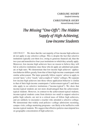
  • 14. 14 Brookings Papers on Economic Activity, Spring 2013 any student whose estimated family income is at or above the cutoff for the top quartile of the same distribution: $120,776. See figure 1 for other percentiles. III.  A Portrait of High-Achieving Students in the U.S. Who and where are the high-achieving students in the United States? In this section, we briefly characterize them, leaving more detailed analysis of the low-income, high-achieving group for later. Figure 2 shows that 34 percent of high achievers have estimated family income in the top quartile and 27 percent have estimated family income in the third quartile. That is, high-income families are overrepresented in the high-achieving population. However, 22 percent and 17 percent of high achievers have estimated family incomes in, respectively, the sec- ond and bottom quartiles. We estimate that there are at least 25,000 and Source: 2008 American Community Survey and authors’ calculations using the combined data set described in the text. a. High-achieving students are defined as in table 2. 1st quartile (17.0%) 2nd quartile (22.0%) 3rd quartile (27.0%) 4th quartile (34.0%) Figure 2.  High-Achieving Students, by Family Income Quartilea
  • 15. caroline hoxby and christopher avery 15 probably about 35,000 low-income high achievers in each cohort in the United States.15 Table 2 shows that among high achievers, those who are from higher- income families do have slightly higher college assessment scores, but the difference is small. The average low-income high achiever scores at the 94.1th percentile. The average high-income high achiever scores at the 95.7th percentile. Data on the parental education of high achievers are unfortunately very incomplete, because ACT takers are not asked to report their parents’ edu- cation, and 52 percent of SAT I takers fail to answer the question about their parents’ education. Moreover, SAT I takers are apparently less likely to report their parents’ education when it is low. We base this assessment on the observation that parents’ education is more likely to be missing for students who live in Census block groups with low adult education. For what they are worth, however, the data on the parents’ education are shown 15. We obtain these numbers by counting the number of high achievers whose esti- mated family income puts them in the bottom quartile of family income. We subtract a number corresponding to our false positive rate and add a number corresponding to our false negative rate. There are two reasons why this procedure gives us a range rather than an exact number. First, many high achievers appear in both the College Board and ACT data. We cannot definitively eliminate all of the duplicates because their names, addresses, and birthdates often do not exactly match in the two data sets. Eliminating all possible duplicates pushes us toward the lower bound. Second, although our false positive rate is robust to the aid data we use, our false negative rate is not. This is because the false nega- tives are low-income students who come from block groups where only a small percentage of families have low incomes. Our aid data from such block groups are fairly sparse, and we are therefore not confident about whether we can extrapolate the false negative rate to areas that appear similar but where we have never observed a false negative. Extrapolating pushes us toward the upper bound. Table 2.  College Assessment Results of High-Achieving Students, by Family Incomea Income quartile Average SAT or ACT percentile score among high-achieving students First (bottom) 94.1 Second 94.3 Third 94.8 Fourth 95.7 Source: Authors’ calculations using data from the ACT, the College Board, IPEDS, and other sources described in the text (hereafter referred to as the “combined data set”). a. High-achieving students are students in 12th grade who have an ACT comprehensive or SAT I (math plus verbal) score at or above the 90th percentile and a high school grade point average of A- or above.
  • 16. 16 Brookings Papers on Economic Activity, Spring 2013 in figure 3.16 More precisely, we show the greater of the father’s reported educational attainment and the mother’s reported educational attainment. Of students who report their parents’ education, 50.7 percent say that at least one parent has a graduate degree, 27.9 percent say that at least one parent has a baccalaureate degree, and another 6 percent cite “some gradu- ate school” (but no degree); 11.6 percent claim that at least one parent has an associate’s degree or “some college or trade school” (but no degree), and only 3.8 percent report neither parent having more than a high school Source: Authors’ calculations using the combined data set described in the text. a. Parents’ educational attainment is the highest level attained by either parent. Percentages are of those high-achieving students (defined as in table 2) who took a College Board test and answered the question about parents’ education (61 percent of high achievers declined to answer; the ACT questionnaire does not include a similar question). Grades 8 or below 0.2% Grades 9–11 0.4% High school diploma 3.2% Some college or trade school 7.4% Associate’s degree 4.2% Bachelor’s degree 27.9% Some graduate school 6.0% Graduate degree 50.7% Figure 3.  High-Achieving Students, by Parents’ Educational Attainmenta 16.  We do not attempt to correct these data for biases because we do not have verified data on parents’ education that we could use to estimate the errors accurately. This is in contrast to family incomes, where we do have a source of verified data (the CSS Profile).
  • 17. caroline hoxby and christopher avery 17 diploma. Perhaps the most interesting thing about the parents’ education data is that they seem to indicate that high achievers are reluctant to report that they have poorly educated parents. This is in contrast to the family income data from the same College Board questionnaire. Many students did not answer the income question, but those who did answered it in an unbiased (albeit fairly inaccurate) way. Figure 4 displays information on high achievers’ race and ethnicity, which 98 percent of students voluntarily report on the ACT or the Col- lege Board questionnaire. Of all high achievers, 75.8 percent say that they are white non-Hispanic, and another 15.0 percent say that they are Asian. The remaining 9.2 percent of high achievers are associated with an under- represented minority,17 either Hispanic (4.7 percent), black non-Hispanic Source: Authors’ calculations using the combined data set described in the text. a. Percentages are of those high-achieving students (defined as in table 2) who took an ACT or a College Board test and answered the question about their race or ethnicity (2.1 percent of high achievers declined to answer). Native American 0.4% Asian 15.0% Black, non-Hispanic 1.5% Hispanic 4.7% White, non-Hispanic 75.8% Mixed 2.6% Figure 4.  High-Achieving Students, by Race and Ethnicitya 17. “Underrepresented minority” is the term of art in college admissions. Notably, it excludes Asians.
  • 18. 18 Brookings Papers on Economic Activity, Spring 2013 (1.5 percent), Native American (0.4 percent), or mixed race/ethnicity (2.6 percent). If we focus on low-income high achievers only (figure 5), we see that 15.4 percent are underrepresented minorities. Interestingly, the entire increase in this share comes out of the percentage who are white. Asians make up 15.2 percent of low-income high achievers, almost identi- cal to their share of all high achievers. A key takeaway from figure 5 is that a student’s being an underrepre- sented minority is not a good proxy for his or her being low-income. Thus, if a college wants its student body to exhibit income diversity commensu- rate with the income diversity among high achievers, it cannot possibly attain this goal simply by recruiting students who are underrepresented minorities. If admissions staff do most of their outreach to low-income students by visiting schools that are largely Hispanic and black, the staff should realize that this strategy may lead to a student body that is diverse on specific racial and ethnic dimensions but that is not diverse in terms of family income. Source: Authors’ calculations using the combined data set described in the text. a. Percentages are of those high-achieving students (defined as in table 2) from bottom-quartile-income families who took an ACT or a College Board test and answered the question about their race or ethnicity (2.1 percent of all high achievers declined to answer). Native American 0.7% Asian 15.2% Black, non-Hispanic 5.7% Hispanic 7.6% White, non-Hispanic 69.4% Mixed 1.4% Figure 5.  High-Achieving, Low-Income Students, by Race and Ethnicitya
  • 19. caroline hoxby and christopher avery 19 Figure 6 is a choropleth map showing the number of high-achieving students in each county of the United States. Counties are an imperfect unit of observation because some are large in land area and some are small. Nevertheless, they are the most consistent political units in the United States.18 The darker is the county’s coloring, the more high-achieving students it contains. What the map demonstrates is that critical masses of high-achieving students are most likely to be found in the urban coun- ties in southern New England (Massachusetts, Connecticut, Rhode Island), the Mid-Atlantic (New York, New Jersey, eastern Pennsylvania), south- ern Florida, and coastal California from the Bay Area to San Diego. The other critical masses are more scattered, but a person familiar with U.S. geography can pick out Chicago (especially), Houston, Dallas-Fort Worth, Atlanta, and some smaller cities. In short, if one’s goal were to visit every county where one could gather at least 100 high achievers, one could con- centrate entirely on a limited number of cities on the East and West Coasts and a few cities in between. Source: Authors’ calculations using the combined data set described in the text. a. Counties are ranked by the absolute number of high achievers (as defined in table 2) living in the county in 2008 and then grouped into deciles; counties are then shaded according to their decile. Most Fewest Figure 6.  Numbers of High-Achieving Students, by Countya 18.  That is, the size and scope of municipalities, school districts, and other jurisdictions are far less consistent than those of counties.
  • 20. 20 Brookings Papers on Economic Activity, Spring 2013 Some part of the above statement is due to the fact that high-income, highly educated parents are somewhat concentrated in the aforementioned areas, and such parents, as we have shown, are somewhat more likely to have high-achieving children. However, some part of the above statement is due purely to population density. That is, even if children in all coun- ties were equally likely to be high-achieving, there would still be critical masses of them in densely populated counties, and vice versa. The choro- pleth map in figure 7 illustrates the role of population density by showing the number of high-achieving students per 17-year-old in each county. The darker a county is, the higher is its decile on this relative measure. The map makes it clear that this relative measure is far less concentrated than the absolute measure that favors densely populated counties. In fact, one can see a belt of counties that tend to produce high achievers running from Minnesota and the Dakotas south through Missouri and Kansas. A good number of counties in Appalachia, Indiana, and the West outside of coastal California also tend to produce high achievers. In short, if one’s goal were to meet a nationally representative sample of high achievers, one’s trip could not be concentrated on a limited number of counties on the coasts and a few cities in between. Source: Authors’ calculations using the combined data set described in the text. a. Counties are ranked by the number of high achievers (as defined in table 2) living in the county in 2008 divided by the number of 17-year-olds living in the county, and then grouped into deciles; counties are then shaded according to their decile. Highest Lowest Figure 7.  Shares of All 17-Year-Olds Who Are High-Achieving, by Countya
  • 21. caroline hoxby and christopher avery 21 IV. College Applications, Enrollment, and Degree Receipt among High-Achieving Students in the U.S. In this section, we analyze the college application choices, enrollment decisions, and on-time degree receipt of high-achieving students in the United States, paying attention to how low-income students’ behavior does or does not differ from that of high-income students. Because colleges in the United States are so varied and large in number, we characterize them by the college assessment score of their median student, expressed as a percentile of the national college assessment test score distribution. This statistic, although admittedly insufficient to describe colleges fully, has important qualities. First, it is probably the single best, simple indicator of selectivity—much better than a college’s admissions rate, for instance (Avery, Glickman, Hoxby, and Metrick, 2013). Second, when an expert college counselor advises students on how to choose a portfolio of schools to which to apply, he or she usually tells students to apply to a few schools that are a “reach,” four or more schools that are “peer” or “match,” and one or more schools that are “safe.” Similar advice is widely available on the Internet sites of college advising organizations with a strong reputa- tion, including the College Board and the ACT. Expert college counsel- ors use schools’ median test scores to define “reach” schools (typically, those whose median score is more than 5 percentiles above the student’s own), “peer” schools (typically, those where the school’s median score is within 5 percentiles of the student’s own), and “safety” schools (typi- cally, those whose median score is 5 to 15 percentiles below the student’s own).19 Naturally, the exact cutoffs for these categories vary from expert to expert, and high-achieving students are often advised to apply to their state’s public flagship university, even if it falls below the safety zone.20 High-achieving students are generally advised to apply to at least eight schools. 19.  Experts also advise students to look at the high school grade point average that is typical of a college’s students. However, such grade-based categories are not terribly relevant to high-achieving students because selective colleges vary so much more on the basis of col- lege aptitude test scores than on the basis of high school grades. 20.  State flagship universities are something of a special case. On the one hand, they vary widely in selectivity. On the other hand, even flagships with low overall selectivity can create opportunities (formal or informal) for their highest-aptitude students to get an education ori- ented to students with their level of achievement. These opportunities may include research jobs and taking courses primarily intended for doctoral students.
  • 22. 22 Brookings Papers on Economic Activity, Spring 2013 IV.A.  College Application Behavior: A Graphical Analysis In this subsection, we provide graphical evidence of what students’ application portfolios look like. This presentation is somewhat informal but useful for fixing ideas and defining categories before we move to the formal econometric analysis in the next subsection. In what follows, an “application” is defined as sending a test score to a college.21 Figure 8 is a histogram of the application portfolios of high-income stu- dents. It is important to understand how this and subsequent figures are constructed. On the horizontal axis is the difference between the applied- to college’s median test score and the student’s own score, in percentiles. Thus, if an application is located at zero, the student is applying to a peer school whose median student has exactly the same score. An application at, say, +8 is a reach, and an application at, say, -13 is a safety. Since nonselec- tive colleges do not require their students to take college assessments (and thus do not report a median student score), an application to a nonselective school is placed at -94, which is zero minus the average percentile score of high-achieving students in the data. It is not obvious where to place applications to nonselective schools, but -94 has the advantage that such applications cannot be mistaken for applications to a school that is selective but that sets a very low bar. Each student is given a weight of 1 in the histogram, and this weight is split evenly over that student’s applications. This is to ensure that the histogram does not overrepresent the behavior of students who apply to more schools, since, after all, each student will enroll at just one (initially at least). Thus, if a student puts all of his or her eggs in one basket and applies to a single +8 school, that student’s full weight of 1 will show up in the +8 bar. If a student applies to one +8 school, one +6 school, one +4 school, and so on down to one -8 school, one 9th of that student’s weight will show up in each of the relevant bars. Note that each bar is 2 percentiles wide. 21.  As noted above, a student may often apply to a nonselective college without sending scores, although a good number of students send scores to them for apparently no reason (the first few sends are free) or for placement purposes (that is, to avoid being placed in lower-level or even remedial courses). If we match students to their enrollment records in the National Student Clearinghouse, we can add to their set of applications any nonselec- tive school in which they enrolled without sending scores. This does not change the figures much, although it does systemically raise the bar for nonselective applications. We do add applications in this way for the analysis in the second half of this section, but it makes too little difference here to be worthwhile, especially as we would then have to show figures for a sample of the students, rather than the population of them.
  • 23. caroline hoxby and christopher avery 23 Figure 8 shows that high-income students largely follow the advice of expert counselors. The bulk of their applications are made to peer schools. They apply to some reach schools as well, but they are mechanically lim- ited in the extent to which they can do this: there are no reach schools for slightly more than half of the high-achieving students we study.22 High-income high achievers also apply fairly frequently to safety schools. Source: Authors’ calculations using the combined data set described in the text. a. The heights of the bars are determined as follows. Each high-income high achiever is assigned a weight of 1, which is divided equally among his or her college applications. Each application is then placed in the vertical bar associated with the difference between the college’s median test score and the applicant’s score. The weights of all applications in a bar are added up, and the resulting sum is the height of the bar. The figure thus depicts the distribution of these students’ applications in the aggregate among the colleges to which they applied. See the text for further details. High-achieving students are defined as in table 2; high-income students are those in the top quartile of the family income distribution (figure 1). –80 –60 –40 –20 –10 0 10 College’s median SAT or ACT score minus student’s score (both in percentiles) 35 40 30 25 20 15 10 5 Percent Figure 8.  Distribution of High-Achieving, High-Income Students’ College Applications, by Student-College Matcha 22.  For instance, consider a student whose own scores put him or her at the 94th per- centile. In order to apply to a reach school, he or she would need to apply to a school whose median student scored at the 99th percentile. There are no such schools—or at least no schools that admit to having such a high median score.
  • 24. 24 Brookings Papers on Economic Activity, Spring 2013 Although not shown in the figure, it is noteworthy that many such stu- dents apply to their state’s flagship university. These schools vary greatly in selectivity, so that some such applications are in the safe range, but other applications to flagships appear far more safe than anyone would think nec- essary. For instance, an application by a high achiever to a flagship with a median score at the 50th percentile would end up at -40 to -50. Neverthe- less, applying to these schools may be well-advised (see note 20). The reader might be surprised to find that high-achieving, high-income students apply to some colleges that are nonselective on academic grounds. However, the schools in question are often specialty schools: music conser- vatories, art or design schools, drama or performing arts schools, cooking schools, and so on. Some of these are highly selective on nonacademic dimensions. Figure 9 shows that unlike the high-income high achievers, few low- income high achievers follow the advice of expert counselors. More than Source: Authors’ calculations using the combined data set described in the text. a. The figure is constructed in a manner analogous to figure 8. –80 –60 –40 –20 –10 0 10 College’s median SAT or ACT score minus student’s score (both in percentiles) 35 40 30 25 20 15 10 5 Percent Figure 9.  Distribution of High-Achieving, Low-Income Students’ College Applications, by Student-College Matcha
  • 25. caroline hoxby and christopher avery 25 40 percent of the mass in the histogram loads on nonselective schools. (This is an underestimate because scores are not sent to some nonselec- tive schools. If we included every nonselective enrollment as a nonselective application, the nonselective bar on the histogram would rise by 5.1 percent- age points.)23 Moreover, the nonselective colleges to which low-income students apply are rarely of the specialty type mentioned above. They are often local community colleges or local 4-year institutions with mea- ger resources per student and low graduation rates. Much of the height of the nonselective bar is due to the fact that many low-income high achiev- ers apply only to nonselective colleges, or to a nonselective college and a barely selective college. Figure 10 overlays the histograms for low-income, middle-income, and high-income students who are high-achieving. It cuts off the portion of the histogram that shows nonselective colleges so as to focus on application choices among colleges that are selective to at least some degree. It will be observed that the behavior of the middle-income students (those from families in the two middle quartiles of the family income distribution) is about midway between that of their low- and high-income counterparts. Moreover, even within the subset of applications that are made to selective colleges, high-income students apply much more to peer colleges, and low- income students apply much more to colleges far below the safety level. Figure 11 contains four panels. The top left-hand panel shows, for all high-achieving, low-income students, the histogram of the most selective college to which each student applied. The top right-hand panel shows the same histogram for high-achieving, high-income students. The bottom left- hand panel shows the histogram for the second most selective college to which a low-income student applied (or the most selective, for students who applied to a single college). The bottom right-hand panel shows the same histogram for high-income students. These histograms reveal that the vast majority of high-income high achievers’ most selective applications fall within 10 percentiles of their test scores. Their second most selective appli- cations are sent to less competitive, but not much less competitive schools: the vast majority fall between +10 and -15 percentiles. In contrast, low- income high achievers send their most selective applications to the entire 23.  We do not treat the sending of no scores as equivalent to applying to no selective institution. The reason is that a student may send no scores because he or she takes both the SAT and the ACT and prefers to send the scores from only one of the two tests. Since we can- not definitively match students across the two data sources (see note 15), we cannot assume that no-score-sending corresponds to no selective applications.
  • 26. 26 Brookings Papers on Economic Activity, Spring 2013 range of colleges: nonselective and -60 to +10. Their second most selective applications are, again, to less competitive (but not necessarily much less competitive) schools. All of this suggests that there may be two distinguish- able types of low-income high achievers: those who apply much as their high-income counterparts do, and those who apply in a manner that is very different. In fact, 53 percent of low-income high achievers fit the profile we will hereafter describe as income-typical: they apply to no school whose median score is within 15 percentiles of their own, and they do apply to at least one nonselective college. At the other extreme, 8 percent of low-income high achievers apply in a manner that is similar to what is recommended and to what their high-income counterparts do: they apply to at least one peer college, at least one safety college with a median score not more than 15 percentiles lower than their own, and apply to no nonselective colleges. Source: Authors’ calculations using the combined data set described in the text. a. The figure is constructed in a manner analogous to figure 8, truncating the left tail of the distribu- tion.The bars for middle-income students are to be read as extending downward to zero behind the low-income bars, and the high-income behind the middle-income. College’s median ACT or SAT score minus student’s score (both in percentiles) 8 6 4 2 Percent –60 –40 –20 –10 0 10 Low-income Middle-income High-income Figure 10.  Distribution of All High-Achieving Students’ College Applications to Selective Institutions, by Student-College Matcha
  • 27. caroline hoxby and christopher avery 27 We hereafter designate such students as achievement-typical, noting that once a student fits the above criteria, he or she usually applies to several peer colleges, much as high-income students do. The remaining 39 percent of low-income, high achievers use applica- tion strategies that an expert would probably regard as odd. For instance, we see some students apply to only a local nonselective college and one extremely selective and well-known college—Harvard, for instance. No expert would advise such a strategy because the probability of getting into Source: Authors’ calculations using the combined data set described in the text. a. Each panel is constructed in a manner analogous to figure 8. –80 –60 –40 –20 –10 0 10 –80 –60 –40 –20 –10 0 10 –80 –60 –40 –20 –10 0 10 –80 –60 –40 –20 –10 0 10 College’s median test score minus student’s score College’s median test score minus student’s score College’s median test score minus student’s score Low-income, second most selective application High-income, second most selective application Low-income, most selective application High-income, most selective application College’s median test score minus student’s score 40 30 20 10 40 Percent Percent Percent Percent 30 20 10 40 30 20 10 40 30 20 10 Figure 11.  Distributions of High-Achieving Students’ Most Selective and Second Most Selective College Applications, by Family Incomea
  • 28. 28 Brookings Papers on Economic Activity, Spring 2013 an extremely selective, well-known college is low if a student applies to just one—even if the student’s test scores and grades are typical of the college’s students. Moreover, such a strategy reveals that the student is interested in extremely selective institutions yet is not applying to the other schools that are, for most purposes, indistinguishable from the one to which he or she applied. Another strategy that appears is a student applying to a single public college in his or her state that is selective but is much less selective than the state’s flagship university. Although about half of these application choices could be motivated by distance from home, the other half cannot because the flagship university is nearer. Another strategy that falls into the idiosyncratic category is a student applying to a single private college outside his or her state that is selective, but much less selective and much poorer in resources than the student’s private peer colleges would be. Such choices are odd because although the private peer colleges might offer fewer scholarships that are explicitly merit-based, they offer much more generous need-based aid, so that the student would pay less to attend and would enjoy substantially more resources. Furthermore, it is almost never sensible for a low-income student to apply to a single private, selec- tive college: such a student can use competing aid offers to improve the aid package at his or her most preferred college. We have described a few salient strategies that appear among low- income high achievers who are neither achievement-typical nor income- typical. However, most of these students’ portfolios do not evince any pattern that can be readily described. Thus, below we turn to an economet- ric analysis, in which we can simultaneously consider a large number of factors correlated with students’ application choices. IV.B.  College Application Behavior: An Econometric Analysis In this subsection we assess the factors that are associated with a stu- dent’s choice of his or her application portfolio, using a conditional logit model in which a student can apply to all colleges in the United States but decides to apply only to some. This model is based on a random util- ity framework and assumes that the student prefers all colleges to which he or she applies over the colleges to which he or she does not apply. We do not assume anything about the student’s preference ordering within the colleges to which he or she applied.24 Each possible college matched with 24.  We considered estimating a rank-ordered logit model (Beggs, Cardell, and Hausman 1981), on the assumption that the order in which the student sent scores to colleges indicates
  • 29. caroline hoxby and christopher avery 29 each student is an observation, and the dependent variable is a binary vari- able equal to 1 if the student submits an application to the college and zero otherwise. The explanatory variables we consider are the difference between a school’s median test score and the student’s own test score if positive, the same difference if negative,25 an indicator for the school’s being nonselec- tive, the distance between the student’s home and the school, the square of this distance, an indicator for the school being the most proximate, an indi- cator for the school being public, an indicator for the school being in-state for the student, an indicator for the school being the flagship university of the student’s state of residence, the sticker price of the college, the likely net cost of the college for the student, and the student-oriented resources per student at the college. We fully interact these explanatory variables with indicators for the student being low-income, high-income, or in between. Thus, we estimate separate coefficients for each income group. In the tables we do not show the coefficients for the middle-income group because they nearly always fall between those of the high- and low-income students, but the coefficients are available upon request. Table 3 shows the results of this estimation. The coefficients are expressed as odds ratios so that a coefficient greater than 1 means that an increase in the covariate is associated with an increase in the probability that the student applies to the school, all other covariates held constant. Based on our graphical analysis, we expect to find very different coeffi- cients for low- and high-income students, and we do.26 Note that, although it is convenient to describe the coefficients as though they literally revealed the rank order of his or her preference among them. (All colleges to which no application is sent are assumed to generate net utility below the bottom-ranked college.) If we do this, the rank-ordered logit generates fairly similar results, in part because many students do not send scores to more than a few colleges. However, the order of score sending might be a poor proxy for some students’ preference orderings because they choose a first batch of colleges to receive their scores before they know what those scores are. Once they learn their scores, they choose a second batch of colleges to receive their scores. At application time, they pre- sumably prefer the second batch to the first. 25.  That is, we do not assume that the response of a student to mismatch is symmetric around his or her own test score. A student may only slightly like being at a reach school, for instance, but strongly dislike being at a safety school. 26. In Avery and Hoxby (2004), we found much smaller differences in the behavior of low- and high-income students, but all the students we sampled attended high schools that were at least somewhat reliable feeders. As we will show, the low-income students we sampled were thus very disproportionately what we call “achievement-typical” students who do behave fairly similarly to high-income students.
  • 30. 30 Brookings Papers on Economic Activity, Spring 2013 preference, they should not be given such a strong interpretation or a causal interpretation. For instance, students might “disfavor” distance not because distance itself generates negative utility but because distant schools have, say, distinct cultures that the student dislikes. We find that high-income students strongly favor reach colleges and disfavor safety colleges (those for which the score difference is negative). Per percentile of difference, this effect is much stronger on the reach side than on the safety side, but recall that high-achieving students can only reach a bit whereas they can apply to very safe schools. High-income stu- dents strongly dislike nonselective institutions. They also dislike higher net costs but (all else equal) like higher sticker prices. This is probably because higher sticker prices are associated with higher per-student resources, a characteristic they also like. High-income students dislike distance, but the quadratic term indicates that they dislike it only up to a point, after which Table 3.  Conditional Logit Regressions Explaining High-Achieving Students’ College Applicationsa Factor Low-income students High-income students College is a peer schoolb 1.015 76.214*** College is a safety schoolc 3.009*** 14.895*** College is nonselective 0.748*** 1.6e-9*** Tuition before discount (thousands of dollars) 0.865*** 1.176*** Average tuition discount (percent) 1.091** 0.925** Could live at family home (college is 10 miles away) 4.942*** 0.810*** Could go home often (college is 120 miles away) 1.556*** 1.185*** Distance in miles to college 0.996 0.998 Square of (distance in miles/1,000) 1.056** 1.283*** College is in-state 2.595*** 1.206*** College is private 0.838*** 1.002 College is for-profit 0.834*** 0.012*** Highest degree offered is 2-year 0.925** 0.009*** College is a university 0.997 0.567*** College is a liberal arts college 0.717*** 0.973* Source: Authors’ regressions using the combined data set described in the text. a. Results of a conditional logit estimation in which the dependent variable is an indicator equal to 1 if a high-achieving student applies to the college and zero otherwise. Coefficients are expressed as odds ratios, so that a coefficient greater than 1 means that an increase in the covariate is associated with an increase in the probability that the student applies to a college with the indicated factor, all other covariates held constant. High-achieving students are defined as in table 2. Low- and high-income students are those from families in the bottom and top quartiles of the family income distribution, respectively. Asterisks indicate statistical significance at the *10 percent, **5 percent, or ***1 percent level. b. The absolute value of the difference between the college’s median test score and the student’s own is within 5 percentiles. c. The college’s median score is 5 to 15 percentiles below the student’s own
  • 31. caroline hoxby and christopher avery 31 they are fairly indifferent. They have a mild preference for in-state schools and their state’s flagship university. They do not have a statistically signifi- cant preference for publicly controlled schools. The low-income students exhibit several immediate contrasts. Such stu- dents strongly favor nonselective colleges. This was obvious in the graphi- cal evidence. They do not disfavor schools whose median scores are lower than theirs. They slightly disfavor schools with higher sticker prices (recall that these were favored by high-income students) and do not have a pref- erence for net costs that is statistically significantly different from zero. Low-income students do favor schools with higher expenditure per student, but not nearly as much as high-income students do. Distance is strongly disfavored for schools within 100 miles but, thereafter, low-income stu- dents are fairly indifferent to it. Low-income students favor in-state schools somewhat more than high-income students do, but low-income students do not exhibit a preference in favor of their state’s flagship university. They slightly favor publicly controlled colleges. Table 4 repeats the estimation but interacts the covariates with indicators forhigh-incomestudents,middle-incomestudents,low-incomeachievement- typical students, low-income income-typical students, and other low-income students. The estimated coefficients for achievement-typical students are fairly similar to those for high-income students. It is the income-typical students whose coefficients are strikingly different. Of course, these results are somewhat by design, given the way we categorized low-income stu- dents into achievement-typical and income-typical groups. However, the coefficients validate the categorization: achievement-typical students do pursue similar application strategies to high-income students. In the next section we assess which factors predict a student being achievement- typical and which predict a student being income-typical. IV.C.  College Enrollment and Progress toward a Degree In this subsection, we demonstrate that, conditional on applying to a specific college, high- and low-income students thereafter behave similarly. There is no statistically significant difference in their probability of enroll- ing or in their progress toward a degree. To find the first of these results, we estimate a conditional logit model in which the binary outcome is 1 for the college in which the student ini- tially enrolled and zero for all others. Importantly, we limit the student’s choice set to the colleges to which he or she applied. So that the student’s enrollment decision is compared to those of students who applied to the same college, we include a fixed effect for each college. We also include
  • 32. 32 Brookings Papers on Economic Activity, Spring 2013 interactions between these fixed effects and an indicator for a student’s hav- ing high or low income. We then test whether each college’s high-income or low-income interaction is statistically significantly different from zero. Thus, we test, specifically, whether high- and low-income students who apply to the same college are differentially likely to enroll in it. We also estimate a variant of this model in which we include an indi- cator variable for each number of colleges to which the student applied: 1 college, 2 colleges, and so on up to 20 or more colleges. This variant tests whether a high- and a low-income student who apply to the same college Table 4.  Conditional Logit Regressions Explaining Income-Typical and Achievement-Typical Students’ College Applicationsa Low-income students Factor Income- typicalb Achievement- typicalc High-income students College is a peer school 7.21e-8*** 87.808*** 76.214*** College is a safety school 2.142*** 19.817*** 14.895*** College is nonselective 0.795*** 1.04e-8*** 1.6e-9*** Tuition before discount (thousands of dollars) 0.973*** 1.004 1.176*** Average tuition discount (percent) 1.000 1.020* 0.925** Could live at family home (college is 10 miles away) 5.140*** 1.477*** 0.810*** Could go home often (college is 120 miles away) 1.972*** 1.436*** 1.185*** Distance in miles to college 0.999 0.999 0.998 Square of (distance in miles/1,000) 1.042* 1.448*** 1.283*** College is in-state 4.891*** 7.455*** 1.206*** College is private 0.662*** 0.296*** 1.002 College is for-profit 0.806*** 0.001*** 0.012*** Highest degree offered is 2-year 0.855*** 0.016*** 0.009*** College is a university 0.956** 0.861*** 0.567*** College is a liberal arts college 0.515*** 0.167*** 0.973* Source: Authors’ regressions using the combined data set described in the text. a. Results of a conditional logit regression in which the dependent variable is an indicator equal to 1 if a high-achieving student applies to the college and zero otherwise. Coefficients are expressed as odds ratios, so that a coefficient greater than 1 means that an increase in the covariate is associated with an increase in the probability that the student applies to a college with the indicated characteristic, all other covariates held constant. The coefficients for high-income students are repeated from table 3 for ease of comparison. High-achieving students are defined as in table 2. Low- and high-income students are those from families in the bottom and top quartiles of the family income distribution, respectively. Asterisks indicate statistical significance at the *10 percent, **5 percent, or ***1 percent level. b. Those who apply to no school whose median score is within 15 percentiles of their own and apply to at least one nonselective school. c. Those who apply to at least one peer college, at least one safety college with a median score not more than 15 percentiles lower than their own, and no nonselective colleges.
  • 33. caroline hoxby and christopher avery 33 and the same number of colleges are differentially likely to enroll in the college in question. Because so few high-income students apply to nonselective and low- selectivity colleges, many of the high-income × college interactions are dropped by the regression. Therefore, the effect of income on enrolling in such colleges, conditional on having applied, is not identified. Note that the tests subsume colleges’ admissions decisions. That is, if we find that high- and low-income students are equally likely to enroll in a college, conditional on having applied to it and to the same number of colleges, they must be getting treated similarly in the admissions process. Otherwise, they would enroll differentially simply because they had been admitted differentially.27 Moreover, if we find that high- and low-income students are equally likely to enroll in a college, conditional on having applied to it (regardless of the number of colleges to which they applied), not only must they be treated similarly in the admissions process, but they must also typically apply to the same number of colleges.28 Table 5 shows the results from these estimations. The table is organized by colleges’ median test scores, with more selective colleges closer to the top. We find that only very small shares of low- and high-income enroll- ment probabilities (conditional on applying) are statistically significantly different from one another at the 5 percent level. For instance, low-income enrollment probabilities differ from high-income enrollment probabilities in only 4 percent of the colleges that have median scores at the 90th per- centile or above. This is about what one would expect from a test at the 5 percent level. The remaining rows of the table contain similar results, all suggesting that low- and high-income students do not enroll differen- tially, conditional on applying. The results are very similar when the esti- mation includes an indicator for each number of colleges to which a student applies. Our test for differential progress toward a degree, conditional on the school at which a student initially enrolled, is constructed in an analogous way. The dependent variable is now the percentage of coursework toward a 27.  We can interact additional student characteristics that might affect admission—for instance, race and ethnicity—with colleges’ fixed effects. This effectively “soaks up” each college’s preferential admissions standards. However, such a specification does not change the estimated coefficients of interest to a noticeable extent, and it makes interpretation slightly harder. 28.  This is a somewhat subtle test of whether the achievement-typical students have total application portfolios like those of high-income high achievers.
  • 34. 34 Brookings Papers on Economic Activity, Spring 2013 4-year degree that the student appears to have completed as of June 2012.29 A student who is making on-time progress should have completed 100 per- cent of his or her coursework by then. We estimate a fixed effect for every college so that students are compared to others who enrolled in the same school. We interact the fixed effects with high- and low-income indicators, and we test whether these interactions are statistically significantly differ- ent. Again, the effects for nonselective and low-selectivity colleges are not identified because so few high-income students enroll in them. The left-hand column of table 6, which is organized in much the same way as table 5, shows the results from this estimation. For selective col- leges, we find that only very small shares of colleges have statistically Table 5.  Estimates Showing Whether High-Achieving, Low- and High-Income Applicants Have Different Probabilities of Enrolling in Selective Collegesa Percent of colleges where low- and high-income students’ probabilities of enrolling (conditional on application) are statistically significantly different at the 5 percent level College’s median test score Base specificationb Base specification plus indicator variables for number of applications sentc ≥90th percentile 4 5 ≥80th but 90th percentile 5 5 ≥70th but 80th percentile 4 5 ≥60th but 70th percentile 3 4 ≥50th but 60th percentile 6 5 50th but college is selective Not identifiedd College is nonselective Not identified Source: Authors’ calculations using the combined data set described in the text. a. Results of a conditional logit estimation in which the dependent variable is an indicator equal to 1 if a high-achieving student enrolls in a particular postsecondary institution and zero otherwise. Each student’s choice set is the set of colleges to which he or she applied. High-achieving students are defined as in table 2. Low- and high-income students are those from families in the bottom and top quartiles of the family income distribution, respectively. b. The only independent variables are indicators for each college interacted with an indicator for whether the student is high- or low-income. c. Indicator variables for whether the student applied to 1 college, 2 colleges, and so on up to 20 or more colleges are added to the specification in the previous column. d. Results are not identified for low-selectivity and nonselective colleges because too few high-income students apply to such colleges. 29.  We do not consider progress toward a 2-year degree because virtually none of the high-achieving students reported that a 2-year degree was their educational goal in the descriptive questionnaires that accompany the ACT and SAT I tests.
  • 35. caroline hoxby and christopher avery 35 significant differences between the progress of their low- and of their high- income students. For instance, low-income students’ progress toward a degree differs from high-income students’ progress toward a degree at only 5 percent of the colleges that have median scores at the 90th percentile or above. This is what one would expect from a test at the 5 percent level. The right-hand column of table 6 reports results of reestimating the model excluding low-income students who attend selective and magnet high schools. The reestimation addresses the possibility that achievement- typical students perform well in college because, although poor, they attended high schools that offer unusually strong preparation. (This is true of some but not most achievement-typical students, as shown below.) We obtain very similar results. There are two key takeaways from this subsection. First, the applica- tion stage is where interesting differences appear in the behavior of high- income high achievers and low-income high achievers. If they apply to the Table 6.  Estimates of Whether Low- and High-Income Students Have Different Probabilities of Persisting at a Selective College, Conditional on Having Enrolleda Percent of colleges where low- and high-income students’ shares of credits earned toward a degree (conditional on enrollment) are statistically significantly different at the 5 percent level College’s median test score Base specificationb Excluding students from selective and magnet high schoolsc ≥90th percentile 5 4 ≥80th but 90th percentile 4 5 ≥70th but 80th percentile 4 5 ≥60th but 70th percentile 5 5 ≥50th but 60th percentile 4 4 50th but college is selective Not identifiedd College is nonselective Not identified Source: Authors’ calculations using the combined data set described in the text. a. Results of an ordinary least squares regression in which the dependent variable is the share of credits toward a baccalaureate degree earned by a student by June 2012. Students who do not enroll in a postsec- ondary institution are not included in the regression. High-achieving students are defined as in table 2. Low- and high-income students are those from families in the bottom and top quartiles of the family income distribution, respectively. b. The only independent variables are indicators for each college interacted with an indicator for whether the student is high- or low-income. c. Same specification as in the previous column, but students who attended high schools classified as magnet schools or that select incoming students on the basis of test scores or grades are excluded. d. Results are not identified for low-selectivity and nonselective colleges because too few high-income students apply to such colleges.
  • 36. 36 Brookings Papers on Economic Activity, Spring 2013 same colleges, their educational paths are similar afterward. Thus, inter- ventions that could make low-income high achievers’ college careers look more like those of their high-income counterparts must, as a logical mat- ter, be focused on the application stage or preparation for it. Second, the data do not suggest that low-income students who currently fail to apply to selective colleges and therefore fail to attend one would be rejected or would perform badly if they were admitted and enrolled. Of course, we cannot say that they would do just as well as the low-income students who do apply. One would need to induce low-income students to apply to sub- stantially more selective schools and then estimate causal effects to make such a claim. We do not attempt to do that in this paper.30 However, we are certainly not struck by evidence that low-income students have poor out- comes when they apply to selective schools. V. Factors That Predict a Student’s Being Achievement-Typical or Income-Typical In this section, we use simple descriptive statistics to identify some fac- tors that predict whether a low-income student is achievement-typical or income-typical. Our goal in this section is to characterize the two types of low-income students sufficiently well that we can build hypotheses about why they apply to colleges so differently. Ex ante, our hypotheses fall into three broad categories: (i)  Despite the fact that both income-typical and achievement-typical students have estimated family incomes in the bottom quartile, income- typical students are actually socioeconomically disadvantaged compared to achievement-typical students when we examine their backgrounds more carefully. Given their greater disadvantage, they cannot be expected to behave similarly. (ii)  Income-typical students are likely to be poorly informed about col- lege compared to achievement-typical students. (iii)  Income-typical students are making rational, well-informed choices about college. Their utility from attending nonselective or less selec- tive colleges exceeds the utility they would derive from attending more selective colleges. 30. Hoxby and Turner (2013) implement exactly the causal test needed by inducing income-typical students to apply to substantially more selective institutions. That study finds no evidence that the students thus induced fail to be admitted at normal rates, fail to attain normal grades, or fail to persist at normal levels.
  • 37. caroline hoxby and christopher avery 37 We can look for evidence of hypotheses in categories (i) and (ii). The hypothesis in category (iii) is inherently untestable, so it is effectively the residual explanation if there is no evidence for other hypotheses. Note that if hypothesis (iii) is the true one, students need not get more utility from attending a nonselective college because it is a good academic match for them. A student might attend a school that is obviously a poor academic match because it enables him or her, say, to look after his or her family. The student might derive sufficient utility from doing this so that his or her college choice is utility maximizing. Cultural and social factors that deter students from applying would also fall under hypothesis (iii). For instance, a student might feel that he or she would enjoy a better social life if he or she attended school with people from a very similar background. Table 7 reports statistics on several characteristics of the families of high-achieving students that might reveal that income-typical students are truly socioeconomically disadvantaged relative to achievement-typical stu- dents. These statistics tend to go the wrong way for hypotheses of type (i). Income-typical students have slightly higher estimated family income than achievement-typical students do. Their (admittedly very flawed) reports of parents’ education suggest that income-typical students’ parents might have 0.7 years more of education than those of achievement-typical students. Achievement-typical students are more likely to be black or Hispanic, so Table 7.  Socioeconomic Characteristics of High-Achieving Studentsa Low-income students Characteristic High-income students Achievement- typical Income- typical Annual family income (dollars)b 157,569 30,475 32,418 Parents’ education (years)c 18.7 16.0 16.7 Race or ethnicityd (percent of total)   White 74.8 45.1 79.5   Black  2.1 5.2 2.9   Hispanic  5.6 12.6 6.0   Asian 20.5 31.8 7.3 Source: Authors’ calculations using the combined data set described in the text. a. High-achieving students are defined as in table 2. Low- and high-income students are those from families in the bottom and top quartiles of the family income distribution, respectively. Achievement- typical and income-typical students are defined as in table 4. b. Estimated as described in section II. c. Highest level of education attained by either parent, as reported by the student. Such self-reporting of parental education is unreliable because students may be more likely not to report if their parents’ educational attainment is low. d. Self-reported.
  • 38. 38 Brookings Papers on Economic Activity, Spring 2013 they are presumably more, not less, likely to have experienced discrimina- tion or to expect to experience it in college. Table 8 reports statistics on several neighborhood factors that are useful for assessing hypotheses of both types (i) and (ii). A person’s neighbors reveal something about his or her own socioeconomic disadvantage, but they also reveal something about the information he or she is likely to encounter. The statistics show that income-typical and achievement-typical students live in Census block groups with very similar average family income. However, achievement-typical students’ block groups are less white, and more black, Hispanic, and Asian than those of income-typical students. Achievement-typical students also have more baccalaureate degree holders in their block groups, both in absolute number (207 versus 144) and as a share of adults (22.0 percent versus 16.8 percent). This last fact suggests that income-typical students may be less likely to get advice about college from a neighbor with a degree. Table 9 compares the geography of income-typical and achievement- typical students, and the contrast is striking. Sixty-five percent of achievement-typical students live in the main city of an urban area, whereas only 30 percent of income-typical students do. Even within main city resi- dents, achievement-typical students are much more likely to live in a large Table 8.  Socioeconomic Characteristics of the Neighborhoods of High-Achieving Studentsa Low-income students Characteristicb High-income students Achievement- typical Income- typical Annual family income (dollars) 123,684 32,142 31,767 Adjusted gross income (dollars)c 121,448 41.358 37,652 Residents with a B.A. degree   Number 863 207    Percent of all adults 66.7 22.0 16.8 Race or ethnicity (percent of total)   White 86.7 58.2 77.1   Black 2.6 12.8 10.1   Hispanic 4.1 16.9 8.7   Asian 9.2 8.5 2.2 Source: Authors’ calculations using the combined data set described in the text. a. High-achieving students are defined as in table 2. Low- and high-income students are those from families in the bottom and top quartiles of the family income distribution, respectively. Achievement- typical and income-typical students are defined as in table 4. b. Neighborhoods are census block groups except where noted otherwise. c. Neighborhood is the ZIP code.
  • 39. caroline hoxby and christopher avery 39 urban area (one with population greater than 250,000). Indeed, 70 percent of the achievement-typical students come from just 15 metropolitan areas (out of 334 nationwide): San Francisco, Oakland, Los Angeles, San Diego, Dallas, Houston, Chicago, Cleveland, Pittsburgh, Portland (Maine), Bos- ton, Providence, New York, Philadelphia, and Baltimore.31 Only 21 percent of achievement-typical students live in a nonurban area (not necessarily rural, but a town rather than an urban-area suburb). By contrast, 47 percent of income-typical students live in a nonurban area. Put another way, income-typical students tend to be the high achievers who live in counties that have a large number of high achievers per 17-year-old (figure 7) but not a large number of achievers in absolute terms (figure 6). Using administrative data from the U.S. Department of Education, table 10 compares the high schools attended by income-typical and achievement- Table 9.  Types of Communities Where High-Achieving Students Residea Percent Low-income students Community type High-income students Achievement- typical Income- typical Main city, urban area with population 250,000 17 26 8 Main city, urban area with population 100,000–250,000 14 21 13 Main city, urban area with population 100,000 48 18 9 Suburb, urban area with population 250,000 8 9 9 Suburb, urban area with population 100,000–250,000 0 2 2 Suburb, urban area with population 100,000 0 4 12 Town, near an urban area 0 5 12 Town, far from an urban area 5 7 13 Rural, near an urban area 6 4 10 Rural, far from an urban area 0 5 10 Source: Authors’ calculations using the combined data set described in the text. a. High-achieving students are defined as in table 2. Low- and high-income students are those from families in the bottom and top quartiles of the family income distribution, respectively. Achievement- typical and income-typical students are defined as in table 4. 31. There were 334 metropolitan statistical areas and primary metropolitan statistical areas in the 2000 Census of Population.
  • 40. 40 Brookings Papers on Economic Activity, Spring 2013 typical students. These statistics should help us to assess these students’ academic disadvantages and the amount of college-related information they might obtain at school. Achievement-typical students are consider- ably more likely to attend a school that is classified as a magnet school or an independent (as opposed to religious) private school. These statistics certainly understate the extent to which the achievement-typical students attend high schools that admit students on the basis of exams or grades. Chester Finn and Jessica Hockett (2012) find that only a small share of such high schools are classified as magnet schools.32 Spending per pupil at achievement-typical students’ public schools is higher, but since facilities and staff costs are often higher in the urban areas where they tend to live, it is unclear whether the higher spending actually gives them an advantage. Pupil-teacher and pupil-counselor ratios are fairly similar for achievement- typical and income-typical students: 18.3 versus 17.2, and 328 versus 305. Using survey data from the Schools and Staffing Surveys from 1987 to 2007 and data on previous cohorts from the College Board and ACT, Table 10.  Characteristics of High Schools Attended by High-Achieving Studentsa Low-income students Characteristic High-income students Achievement- typical Income- typical Number of students per cohort 333 330 241 Type of school (percent of total)    Regular public school 66 73 86   Magnet school 4 11 0    Independent private school 16 7 3    Catholic or other religious school 15 9 11 Spending per pupil (dollars; public schools only) 15,558 12,975 10,701 Pupil-teacher ratio 16.8 18.3 17.2 Pupil-counselor ratio (public schools only) 307 328 305 Source: Authors’ calculations using the combined data set described in the text. a. High-achieving students are defined as in table 2. Low- and high-income students are those from families in the bottom and top quartiles of the family income distribution, respectively. Achievement- typical and income-typical students are defined as in table 4. 32.  Finn and Hockett found most of the selective high schools in their study by word of mouth and by contacting all high schools that were so dissimilar to other schools in their district that they seemed likely to practice selective admissions. Interestingly, many school districts deemphasize the existence of their selective high schools, which can be controver- sial. This perhaps explains why there was no reasonably accurate list of them before Finn and Hockett (2012).