SlideShare a Scribd company logo
1 of 36
PNGE 441 Project2
1 | P a g e
Project #2
Petroleum and Natural Gas Engineering: 441
12-04-2014
Group 3
Herbert M. Hand Jr., Michael Palma, Haven Williams,
Lyla Almaskeen, Emmanuel Bate, Richard Steinmiller,
Carl Chidester, Mustafa Al Hajji, Maria Mata Madrid,
Jake Duska, and Abdullah Alshabaan
West Virginia University
PNGE 441 Project2
2 | P a g e
Dr. Zamirian,
Group3’s project 2iscontainedunderthisletter. We have collectivelycompletedthewater-flood
scenarios for project 1’s reservoir from 1/1/2014 to 1/1/2024. We assumed that all of the new wellsin
eachcase are drilledinthe fieldatthe same time(1/1/2014). We modeledandraneachscenariobyusing
the CMG IMEX simulator until 1/1/2024. The results for each scenario were exported intoexcel,where
we analyzedthe production. Economicanalysisforeachscenariowas implemented,andwe hadto take
into account the direct costs, investments, income tax, interest rate, and the price of oil and gas with
respect to the change in time. The “Net Cash Flow” method was the basis of our analysis. Once we
correlatedthe variablesandall of the data foreach scenario,we were able to determine whichscenario
was the best for water flooding. In your project description, you asked us the following:
A. For each scenario do the economic analysis and find annual NPV for 6% interest rate.
B. Plot cumulative NPV vs. year for each scenario in the same plot for 6% interest rate.
C. What is the best scenario with 6% interest rate if we plan to produce until:
a. 1/1/2024
b. 1/1/2023
c. 1/1/2022
d. 1/1/2021
e. 1/1/2020
D. And repeat the parts A through C with different interest rates (2%, 10%, 14%, and 18%).
E. Summarize all your answers
F. Plot oil RF vs. NPV for all scenarios in one plot
G. Plot gas RF vs. NPV for all scenarios in one plot
H. Write your conclusions
I. Prepare a presentation in which one group member will present the group work.
All of these were completed and answered to the best of our ability.
- The contents withinthe CDinclude the electronicversionof our Project2Report,the excel spreadsheet
with our economical analysis, the CMG reservoir model (.dat) files for each scenario and case, and the
PowerPointpresentation. If there are problems orquestions,pleasecontactHerbertM. Hand viaemail.
Sincerely,
HerbertM. HandJr.,Michael Palma,HavenWilliams,LylaAlmaskeen,EmmanuelBate,RichardSteinmiller,
Carl Chidester, Mustafa Al Hajji, Maria Mata Madrid, Jake Duska, and Abdullah Alshabaan.
West Virginia University
Petroleum and Natural Gas Engineering
hhand@mix.wvu.edu
PNGE 441 Project2
3 | P a g e
Work Log
 CMG Cases 1 and 2 – Abdullah, Lyla, and Mustafa worked collectively on this for 3 days.
(11/12 – 11/15)
 Economical Analysis – Haven, Jake, Lyla, Richard, Maria, and Michael worked on this.
The first scenario was worked on collectively. Once a generalized table was created,
everyone completed 3 separate scenarios. Then, the PVP, IRR, and RF curves were
generated (11/16-12/03)
 Project Report – Herb wrote this. Lyla and Abdullah helped Herb with the Case 1 and
Case 2 Methodology. Haven, Jake, and Michael helped Herb with the Economic Analysis
Methodology. (11/16-12/03)
 Calculations and Results – Maria, Emmanuel, and Richard worked on analyzing the results,
and were responsible for the writing of the calculations and results section of the project.
This was sent to Herb to include in the project report (11/21-12/03)
 Power Point Presentation – Carl (12/04)
PNGE 441 Project2
4 | P a g e
Project Objectives:
Simulate a water-flood in project 1’s reservoir by (See figure 1)
Decide where to drill the new (producer) wells by analyzing the parameters of the reservoir.
Record the generated data and analyze it in order to predict the production, which, in turn, will
help to predict the economic analysis.
Problem Statement
In Project 2, a team of 9 members are asked to complete an economic analysis of the oil
reservoir from Project 1. The field is water-flooded in order to increase recovery after 15 years of
production (1/1/1999 – 1/1/2014), and it will be water-flooded for the next 10 years (1/1/2014 –
1/1/2024). Two cases are presented to the team (see figure 1.) The first case has 6 injection wells,
and the second case has 9. Each case has 5 scenarios and a different number of added producing
wells. The objectives of the project are to:
A. Simulate a water-flood by using CMG for two different cases with 5 sub-scenarios
a. Run each scenario until 1/1/2024
b. Assume all the new wells are drilled in the field at the same time (1/1/2014)
B. Decide where to drill the new (producer) wells by analyzing the parameters of the reservoir.
C. Record the generated data and analyze it in order to predict the production, which, in turn,
will help to predict the economic analysis.
D. For each scenario, do an economic analysis.
a. Use the “Net Cash Flow” Method
b. Find annual NPV
c. Plot cumulative NPV vs. year for each scenario in the same plot
d. Find the best scenario if we plan to produce until 2024, 2023, 2022, 2021, and 2020.
e. Repeat steps b through d for 4 other situations, where the interest rate changes (2%,
10%, 14%, and 18%)
f. Plot oil RF vs. NPV for each scenario in the same plot
g. Plot gas RF vs. NPV for each scenario in the same plot
Figure 1: Cases 1 and 2. Scenarios 1 through 10 are shown.
PNGE 441 Project2
5 | P a g e
Methodology
This project was heavily reliant on a reservoir model that was generated through the CMG
program, Builder. CMG stands for Computer Modelling Group, and they produce reservoir
simulation programs for the petroleum and natural gas industry. The model, from project 1, was
already built for us, but for each scenario we had to increase the number of producer wells. In
order to do this, the Builder program was implemented. After entering the program, it asks to
define the simulator’s settings. The parameters were set to IMEX simulator, Field units, Single
Porosity, and the start date was set to January 1st, 1999. Hit OK. Next, both case’s models were
uploaded to the program. The model (.dat) files were given to us by Professor Zamirian, and the
following is the methodology to complete the water-flood for case 1, case 2, and all of the sub-
scenarios:
Case 1
1. First, download both case files from eCampus. (Provided by Professor Zamirian)
2. Open PNGE 441 – Project2-Case-1.dat in CMG builder
3. Start with sub scenario 5 (from figure 1). Add 49 producing wells. There will be 67 total
wells (12 first producers from project 1, 6 injection wells, and 49 new producers)
a. Right click on Well-018, and select “New” and you will be prompted to the Create
New Well screen
b. Select “Producer” from the Type dropdown menu.
c. Change definition date to 2014-01-01. Press OK.
d. Repeat 48 more times
4. The constraints need to be modified to the specifications in the project description.
a. Right-click on any of the additional wells, click properties, click constraints, and
from the constraint dropdown menu select “Operate”.
b. Then, select “STW surface water rate” from the parameter drop-down menu, select
“MAX” from the Limit/Mode dropdown menu, Set the value to 200 bbls/day, and
select “Shut In” from the Action dropdown menu. Press apply.
c. Make a new constraint and select “Operate” from the dropdown menu.
d. Then, select “BHP bottom hole pressure” for the Parameter dropdown menu, select
“Min” from the Limit/Mode dropdown menu, set the value to 500 psi, and select
“Shut In” for the Action
e. Now, when the IMEX simulator runs the wells that meet these constraints during
production will be shut in.
f. Repeat step 4 for all additional wells.
5. Next, place each new well in a location in the reservoir
a. Press “Well” at the top of Builder, and then press “Well Completions Perf”
b. On the “Well Completion Data (Perf)” screen select Well-019 and press the
“Perforations” tab.
c. Press insert. Then, in order to choose the User Block Address, press on the “Begin”
button to add perforations with the mouse. Select a block to add the location, and
press “Stop”. You need to do this for both layers
PNGE 441 Project2
6 | P a g e
d. Press insert again to get a new line. Copy the User Block Address from line 1 and
change the last number to a “2”.
e. Note: Well placement optimization is very important. Use engineering judgement
and the 3D result for decision.
6. After all of the wells are drilled, Press “Validate With IMEX”. The program will ask to
save the file. Press “Yes”. Select “Run Normal Immediately” and Press “Run”. Once the
simulator completes, export the data to excel.
7. After scenario 5 is completed, work each other scenario from case one – starting with sub-
scenario 4.
8. For sub-scenario 4, remove 12 wells that are insignificant. Run IMEX and export data to
excel.
9. For sub scenario 3, remove 10 wells that are insignificant. Run IMEX and export data to
excel.
10. For sub scenario 2, remove 5 wells that are insignificant. Run IMEX and export data to
excel.
11. For sub scenario 1, remove 5 wells that are insignificant. Run IMEX and export data to
excel.
Case 2
12. Open PNGE 441 – Project2-Case-2.dat in CMG builder
13. Start with sub scenario 10. Add 49 producing wells. There will be 70 total wells (12 first
producers from project 1, 9 injection wells, and 49 new producers)
a. Right click on Well-021, and select “New” and you will be prompted to the Create
New Well screen
b. Select “Producer” from the Type dropdown menu.
c. Change definition date to 2014-01-01. Press OK.
d. Repeat 48 more times
14. The constraints need to be modified to the specifications in the project description. Follow
step 4.
15. Next, place each new well in a location in the reservoir. These locations will be the same
locations as in Case 1. Follow step 5.
16. After all of the wells are drilled, Press “Validate With IMEX”. The program will ask to
save the file. Press “Yes”. Select “Run Normal Immediately” and Press “Run”. Once the
simulator completes, export data to excel.
17. Then, for sub-scenario 9, remove 12 wells that are insignificant. Run IMEX and export
data to excel (Use the same wells that were removed in Case 1 – sub scenario 4).
18. For Sub Scenario 8, remove 10 wells that are insignificant. Run IMEX and export data to
excel (Use the same wells that were removed in Case 1 – sub scenario 3).
19. For Sub Scenario 7, remove 5 wells that are insignificant. Run IMEX and export data to
excel (Use the same wells that were removed in Case 1 – sub scenario 2).
20. For Sub Scenario 6, remove 5 wells that are insignificant. Run IMEX and export data to
excel (Use the same wells that were removed in Case 1 – sub scenario 1).
PNGE 441 Project2
7 | P a g e
Economic Analysis
21. Open each excel file and create a table for an economic analysis of each scenario and case.
22. Assumptions for the economic analysis are
a. Income Tax = 50%
b. Drilling Cost = $5,000,000 /well
c. Operating Cost (producers) = $4,000,000/year/well with a 4% annual increase from
2014
d. Operating Cost (injectors) = $5,000,000/year/well with a 4% annual increase from
2014
e. Oil Price = $80/STB with a .2% annual increase from previous year
f. Gas Price = $3.5/MSCF with a .1% annual increase from the previous year.
23. Calculate Revenues, Direct Costs, Income Taxes, Net Cash Flow (NCF), Present Value
(PV) for each interest rate (2 %, 10 %, 14%, 18%), and Net Present Value (NPV) for each
interest rate (2 %, 10 %, 14%, 18%) and for each of the 10 years of the water-flood.
a. 𝐺𝑎𝑠 𝑅𝑒𝑣𝑒𝑛𝑢𝑒 (𝐺𝑅𝑡) = 𝑃𝑟𝑖𝑐𝑒 𝑔𝑎𝑠 𝑡
∗
𝐺 𝑝 𝑡
1000
, 𝑤ℎ𝑒𝑟𝑒 𝑡 = 𝑡𝑖𝑚𝑒 ( 𝑦𝑒𝑎𝑟𝑠)
b. 𝑂𝑖𝑙 𝑅𝑒𝑣𝑒𝑛𝑢𝑒 (𝑂𝑅𝑡) = 𝑃𝑟𝑖𝑐𝑒 𝑜𝑖𝑙 𝑡
∗ 𝑁 𝑝 𝑡
c. 𝐷𝑖𝑟𝑒𝑐𝑡 𝐶𝑜𝑠𝑡𝑠(𝐷𝐶𝑡) = 𝑁 𝑝𝑟𝑜𝑑𝑢𝑐𝑖𝑛𝑔 𝑡
∗ 𝑂𝐶 𝑝𝑟𝑜𝑑𝑢𝑐𝑖𝑛𝑔 𝑡
+ 𝑁𝑖𝑛𝑗 𝑡
∗ 𝑂𝐶𝑖𝑛𝑗 𝑡
i. Where N=number of wells and OC = Operating Costs
d. Income Tax (𝐼𝑇𝑡) = ( 𝐺𝑅𝑡 + 𝑂𝑅𝑡 − 𝐷𝐶𝑡) ∗ 50%
e. 𝑁𝐶𝐹𝑡 = 𝐺𝑅𝑡 + 𝑂𝑅𝑡 − 𝐷𝐶𝑡 − 𝐼𝑇𝑡
f. 𝑃𝑉𝑡 =
𝑁𝐶 𝐹𝑡
(1+𝐼𝑅) 𝑡, where IR = Interest Rate
g. 𝑁𝑃𝑉𝑡 = 𝑃𝑉𝑡 + 𝑁𝑃𝑉𝑡−1 , 𝑤ℎ𝑒𝑟𝑒 𝑁𝑃𝑉𝑡−1( 𝑡 = 0) = −𝐼𝑛𝑣𝑒𝑠𝑡𝑚𝑒𝑛𝑡𝑠
h. Do all of these calculations for each case, scenario, interest rate, and year.
24. Plot cumulative NPV vs. t (year) for each scenario in same plot. Make a plot for each
interest rate (2 %, 10 %, 14%, 18%).
25. Next, plot the Present Value Profile (PVP)
a. In addition to the previously calculated interest rates from step 22 and 23, calculate
PV and NPV from arbitrary interest rates until the PV at 10 years for each scenario
reaches a negative value.
b. Then, plot NPV vs. Interest Rate for each scenario. This is your Present Value
Profile.
c. From your PVP plot, you can determine the IRR for each scenario.
d. IRR is the internal rate of return, and is the discount rate when NPV reaches zero
e. Using the equation: 𝑁𝑃𝑉 = ∑
𝑁𝐶 𝐹𝑡
(1+𝐼𝑅𝑅) 𝑡 = 0, 𝑠𝑜𝑙𝑣𝑒 𝑓𝑜𝑟 𝐼𝑅𝑅,𝐿
𝑡=0 and solve the IRR
for each scenario
i. Where L = 10 years
26. Finally, find the oil and gas recovery factor for each sun scenario
a. 𝑂𝑖𝑙 𝑅𝐹 =
𝑁 𝑝
𝑂𝑂𝐼𝑃
, 𝑑𝑜 𝑡ℎ𝑖𝑠 𝑓𝑜𝑟 𝑒𝑎𝑐ℎ 𝑠𝑢𝑏 − 𝑠𝑐𝑒𝑛𝑎𝑟𝑖𝑜′
𝑠 𝑁 𝑝 𝑣𝑎𝑙𝑢𝑒.
b. 𝐺𝑎𝑠 𝑅𝐹 =
𝐺 𝑝
𝑂𝐺𝐼𝑃
, 𝑑𝑜 𝑡ℎ𝑖𝑠 𝑓𝑜𝑟 𝑒𝑎𝑐ℎ 𝑠𝑢𝑏 − 𝑠𝑐𝑒𝑛𝑎𝑟𝑖𝑜′
𝑠 𝐺𝑝 𝑣𝑎𝑙𝑢𝑒.
PNGE 441 Project2
8 | P a g e
Wellbore Placement Optimization
In order to have the optimal recovery for our reservoir, the wells were placed in specific
locations using engineering judgment and the constraints that were given in the project (max
allowable surface water rate is 200 bbls/day and minimum bottom hole pressure is 500 psia).
Initially, 12 producing wells and the injection wells (6 for case 1 and 9 for case 2) were added by
Professor Zamirian. Considering permeability, pay thickness, and porosity, the locations of the
remaining wells were determined. After running the IMEX simulator, it was discovered that
some wells were shut in. This is a result of placing the wells too close to the injection wells. So,
putting this into consideration, the shut in wells were optimally relocated.
Figure 2: Scenario 5 well locations (upside down triangles denote the injection wells)
PNGE 441 Project2
9 | P a g e
Figure 3: Scenario 10 well locations (upside down triangles denote the injection wells)
PNGE 441 Project2
10 | P a g e
Calculations and results
A) For each scenario do the economic analysis and find annual NPV.
B) Plot cumulative NPV vs. year for each scenario in the same plot.
-5E+08
0
500000000
1E+09
1.5E+09
2E+09
2012 2014 2016 2018 2020 2022 2024 2026
NPV
Time (year)
2% Interest Rate
Scenario 1
Scenario 2
Scenario 3
Scenario 4
Scenario 5
Scenario 6
Scenario 7
Scenario 8
Scenario 9
Scenario 10
Figure 4: Each sub-scenario's calculated NPV at a 2% interest rate from Jan 1st 2014 - Jan 1st 2024
PNGE 441 Project2
11 | P a g e
Figure 5: Each sub-scenario's calculated NPV at a 6% interest rate from Jan 1st 2014 - Jan 1st
2024
-5E+08
0
500000000
1E+09
1.5E+09
2E+09
2012 2014 2016 2018 2020 2022 2024 2026
NPV
Time (year)
6% Interest Rate
Scenario 1
Scenario 2
Scenario 3
Scenario 4
Scenario 5
Scenario 6
Scenario 7
Scenario 8
Scenario 9
Scenario 10
PNGE 441 Project2
12 | P a g e
PNGE 441 Project2
13 | P a g e
Figure 6: Each sub-scenario's calculated NPV at a 10% interest rate from Jan 1st 2014 - Jan 1st
2024
-4E+08
-2E+08
0
200000000
400000000
600000000
800000000
1E+09
1.2E+09
1.4E+09
1.6E+09
2012 2014 2016 2018 2020 2022 2024 2026
NPV
Time (year)
10% Interest Rate
Scenario 1
Scenario 2
Scenario 3
Scenario 4
Scenario 5
Scenario 6
Scenario 7
Scenario 8
Scenario 9
Scenario 10
PNGE 441 Project2
14 | P a g e
Figure 7: Each sub-scenario's calculated NPV at a 14% interest rate from Jan 1st 2014 - Jan 1st
2024
-4E+08
-2E+08
0
200000000
400000000
600000000
800000000
1E+09
1.2E+09
1.4E+09
2012 2014 2016 2018 2020 2022 2024 2026
NPV
Time (year)
14% Interest Rate
Scenario 1
Scenario 2
Scenario 3
Scenario 4
Scenario 5
Scenario 6
Scenario 7
Scenario 8
Scenario 9
Scenario 10
PNGE 441 Project2
15 | P a g e
-4E+08
-2E+08
0
200000000
400000000
600000000
800000000
1E+09
1.2E+09
1.4E+09
2012 2014 2016 2018 2020 2022 2024 2026
NPV
Time (year)
18% Interest Rate
Scenario 1
Scenario 2
Scenario 3
Scenario 4
Scenario 5
Scenario 6
Scenario 7
Scenario 8
Scenario 9
Scenario 10
PNGE 441 Project2
16 | P a g e
Figure 8: Each sub-scenario's calculated NPV at a 18% interest rate from Jan 1st 2014 - Jan 1st
2024
The following questions are answered below (see figure 9):
C) What is the best scenario if we plan to produce until 1/1/2024?
D) What is the best scenario if we plan to produce until 1/1/2023?
E) What is the best scenario if we plan to produce until 1/1/2022?
F) What is the best scenario if we plan to produce until 1/1/2021?
G) What is the best scenario if we plan to produce until 1/1/2020?
Year Scen. 1 Scen. 2 Scen. 3 Scen. 4 Scen. 5 Scen. 6 Scen. 7 Scen. 8 Scen. 9 Scen. 10
2014 -115000000 -140000000 -165000000 -215000000 -275000000 -130000000 -155000000 -180000000 -230000000 -290000000
2015 320023580.7 370740884.1 405611020.3 458714303.5 487744662.8 296223296.3 347346040.7 382980003.6 439674293.7 464249927.8
2016 644640325.2 738001411.9 805773509.9 910069898.8 980221621 613938539.9 707587367 777705796.5 889008742 953815310.1
2017 902809910.7 1020471922 1106423935 1236992705 1325336648 867952217.4 985845147.7 1075391369 1216050048 1300610083
2018 1111555360 1240482068 1333365405 1470749691 1557161433 1074302686 1202973451 1300905401 1451020158 1535734681
2019 1280352357 1409116312 1498428432 1624868389 1693051010 1241960183 1370070909 1466354008 1607386297 1676448301
2020 1414862775 1533544245 1610266746 1710943696 1749703805 1376698460 1494726525 1580547012 1696806509 1738670111
2021 1519956243 1620332072 1677926674 1744113360 1746565419 1483419090 1583725731 1652110418 1734011950 1741113517
2022 1598074057 1673739877 1708383180 1736540706 1700690556 1564463343 1641049103 1687369794 1731421408 1700144062
2023 1652124853 1698853846 1708943834 1698931461 1622910674 1622530422 1671337217 1693123040 1699059981 1627702450
2024 1683665965 1700201695 1686072604 1638357737 1521004222 1658952955 1678619901 1675362341 1643799465 1531032382
2% Interest Rate NPV
Figure 9: The best case scenarios according to the year and interest rate. This
is a crucial step to determining the most feasible scenario for your project.
Figure 10: 2% interest rate NPV calculated for each scenario for each year.
Interest 2020 2021 2022 2023 2024
2% 5 4 3 2 1
6% 5 4 3 2 7
10% 5 4 3 2 7
14% 5 4 3 2 7
18% 5 4 3 2 7
Best Scenario
PNGE 441 Project2
17 | P a g e
Year Scen.1 Scen.2 Scen.3 Scen.4 Scen.5 Scen.6 Scen.7 Scen.8 Scen.9 Scen.10
2014 -115000000 -140000000 -165000000 -215000000 -275000000 -130000000 -155000000 -180000000 -230000000 -290000000
2015 303607596.5 351467643.2 384078529 433291122.2 458961845.4 280139398.3 328389586.4 361735475.2 414403565.6 435787666.4
2016 604187216.4 691533372.2 754609905 851224872.1 914972015.6 574328557.7 661955869.6 727232729.5 830465829.8 889101856.2
2017 834219079.6 943217619.5 1022492651 1142516591 1222473197 800657462.3 909886529.6 992473759.9 1121863133 1198099710
2018 1013194851 1131851602 1217069466 1342936945 1421236906 977579806.3 1096049657 1185826707 1323323605 1399692637
2019 1152458012 1270980487 1353251976 1470090019 1533350346 1115902842 1233910641 1322327335 1452330893 1515786074
2020 1259245842 1369763831 1442040422 1538425211 1578327004 1222871569 1332874743 1412985168 1523321605 1565183973
2021 1339531112 1436064660 1493728654 1563764896 1575929461 1304399895 1400864936 1467655429 1551744388 1567050593
2022 1396956578 1475325463 1516117645 1558198135 1542206226 1363976627 1443004126 1493575076 1549840045 1536933389
2023 1435190676 1493090419 1516514237 1531594353 1487186802 1405051738 1464429134 1497644769 1526948431 1485690116
2024 1456660084 1494007873 1500946245 1490363024 1417821106 1429843832 1469386312 1485555414 1489333696 1419888723
6% Interest Rate NPV
Year Scen. 1 Scen. 2 Scen. 3 Scen. 4 Scen. 5 Scen. 6 Scen. 7 Scen. 8 Scen. 9 Scen. 10
2014 -115000000 -140000000 -165000000 -215000000 -275000000 -130000000 -155000000 -180000000 -230000000 -290000000
2015 274231624.8 316978685.8 345546702.4 387797008.4 407455751 251357686.1 294467510.1 323718950.6 369182262.8 384855198.5
2016 534104863.5 610990576.4 665898390.7 749131543.2 801710157.9 505705900.6 582860150.8 639718269.6 728898760.2 776778731.7
2017 719027909.7 813320014.8 881249832.7 983301502.1 1048910935 687652131.5 782172073.4 852946031.3 963153598.5 1025182686
2018 852810099 954321598.2 1026693610 1133113253 1197484364 819899408.9 921326722.6 997474982.8 1113742825 1175870921
2019 949602512.2 1051020685 1121344871 1221488763 1275406841 916038404.5 1017144578 1092347346 1203407074 1256559625
2020 1018615026 1114860234 1178725135 1265650943 1304473376 985167824.3 1081100943 1150935716 1249285406 1288483423
2021 1066858988 1154700851 1209784943 1280877732 1303032676 1034158748 1121956710 1183787446 1266364848 1289605088
2022 1098944771 1176637349 1222294520 1277767372 1284190227 1067446524 1145501472 1198269735 1265300820 1272777465
2023 1118808463 1185866744 1222500561 1263945957 1255606085 1088786202 1156632367 1200384055 1253407981 1246155140
2024 1129179691 1186309939 1214980130 1244028335 1222097592 1100762521 1159027032 1194544049 1235237428 1214368456
14% Interest Rate NPV
Year Scen.1 Scen.2 Scen.3 Scen.4 Scen.5 Scen.6 Scen.7 Scen.8 Scen.9 Scen.10
2014 -115000000 -140000000 -165000000 -215000000 -275000000 -130000000 -155000000 -180000000 -230000000 -290000000
2015 261037332.5 301487882.8 328240034.5 367363211.5 384321657.7 238430306.9 279231323.3 306643732 348870999.6 361978751.1
2016 503590665.5 575904611.6 627241078.8 704615697.4 752299988.1 475826844.9 548403311.2 601582481.5 684613286.4 727781554.7
2017 670338257.5 758347781 821426363.6 915769891.4 975204245.3 639890202.6 728125546 793852815.3 895844017.2 951770732.9
2018 786882191.8 881180867.8 948129253.7 1046277928 1104633522 755097003.3 849349681.9 919758757.7 1027029349 1083042316
2019 868344279.9 962564410.8 1027789313 1120656212 1170214361 836009164.3 929991565.9 999604899.9 1102492257 1150951257
2020 924457463.5 1014471524 1074444464 1156563910 1193847985 892217402.9 981993660.4 1047242347 1139795336 1176908086
2021 962354292.8 1045767317 1098842715 1168524930 1192716279 930700988.9 1014086879 1073048196 1153211662 1177789181
2022 986704092.5 1062414856 1108336193 1166164488 1178416805 955962977.6 1031954925 1084038760 1152404174 1165018751
2023 1001267586 1069181586 1108487256 1156031020 1157459725 971608622.3 1040115781 1085588919 1143684683 1145500020
2024 1008613717 1069495509 1103160398 1141923005 1133725048 980091667.7 1041811965 1081452337 1130814149 1122984931
18% Interest Rate NPV
Figure 11: 6% interest rate NPV calculated for each scenario for each year.
Year Scen. 1 Scen. 2 Scen. 3 Scen. 4 Scen. 5 Scen. 6 Scen. 7 Scen. 8 Scen. 9 Scen. 10
2014 -115000000 -140000000 -165000000 -215000000 -275000000 -130000000 -155000000 -180000000 -230000000 -290000000
2015 288385502.1 333596092.5 364112037 409716899.6 432272323.7 265225238.3 310811783.2 342036003.4 390970708.7 409395387.6
2016 567502246.7 649379442.2 708185635.5 797808107.4 855721106.6 538407833 620559779.8 681434941.3 777324064.1 830340696.5
2017 773341187 874593541 947894603.8 1058464079 1130881758 740933262.5 842415063.8 918780028.5 1038074515 1106840612
2018 927669981.4 1037250502 1115676002 1231284295 1302273468 893491409.4 1002941434 1085506100 1211791614 1280671926
2019 1043388309 1152857255 1228834516 1336939954 1395432203 1008428556 1117494647 1198928948 1318988000 1377137769
2020 1128895146 1231954764 1299928939 1391657109 1431445780 1094080241 1196736892 1271520221 1375831474 1416691510
2021 1190843266 1283112489 1339811583 1411209211 1429595835 1156987503 1249198130 1313703799 1397762496 1418131794
2022 1233541506 1312304541 1356458736 1407070092 1404521197 1201285299 1280530383 1332976142 1396346537 1395738392
2023 1260936390 1325033202 1356742895 1388008375 1365099560 1230715780 1295881487 1335892094 1379944604 1359022381
2024 1275759928 1325666658 1345993986 1359540232 1317206063 1247833465 1299304167 1327545007 1353973536 1313589855
10% Interest Rate NPV
Figure 12: 10% interest rate NPV calculated for each scenario for each year.
Figure 13: 14% interest rate NPV calculated for each scenario for each year.
Figure 14: 18% interest rate NPV calculated for each scenario for each year.
PNGE 441 Project2
18 | P a g e
When selecting the best case scenario for each year at each interest rate, the net present
value (NPV) was taken into account. Along with the highest magnitude NPV value, the slope of
each line is investigated to determine the best case scenario. The scenario with the highest NPV
value and still increasing slope is chosen as the best case scenario for each year and interest rate.
If the slope is decreasing at any time selected, the value of the scenario is already decreasing and
is therefore losing money. When the slope is increasing, the scenario is still increasing in value
and is still an operable scenario. As soon as the slope begins its decline, the scenario is not feasible.
The best case scenarios for each year and interest rate can be found in the table above.
While adding more wells increases recovery factors initially, there is a steep drop off as
time passes. Adding more wells will increase profits in the early stages of production, but will
increase costs later in production. This also pertains to injection wells. As more injection wells
are added, the production rates will increase and recovery factors will be high. But, as time passes,
the recovery factor declines rapidly, and costs will start to overcome profit from production.
Therefore, it is financially smarter to produce with fewer wells.
The oil and gas recovery factors for each scenario vs. time and the oil and gas recovery factors vs.
NPV for each interest rate can be found in the charts below.
Figure 15: Oil recovery factor vs. time
0%
5%
10%
15%
20%
25%
30%
2012 2014 2016 2018 2020 2022 2024 2026
OilRF(%)
Time (years)
Oil Recovery Factor vs. Time
Scenario 1
Scenario 2
Scenario 3
Scenario 4
Scenario 5
Scenario 6
Scenario 7
Scenario 8
Scenario 9
Scenario 10
PNGE 441 Project2
19 | P a g e
Figure 16: Gas recovery factor vs. time
0%
5%
10%
15%
20%
25%
30%
35%
40%
45%
2012 2014 2016 2018 2020 2022 2024 2026
GasRF(%)
Time (years)
Gas Recovery Factor vs. Time
Scenario 1
Scenario 2
Scenario 3
Scenario 4
Scenario 5
Scenario 6
Scenario 7
Scenario 8
Scenario 9
Scenario 10
PNGE 441 Project2
20 | P a g e
Figure 17: Oil RF vs. NPV at 2% interest
-5E+08
0
500000000
1E+09
1.5E+09
2E+09
15% 17% 19% 21% 23% 25% 27% 29%
NPV
Oil RF
2% Interest Rate
Scenario 1
Scenario 2
Scenario 3
Scenario 4
Scenario 5
Scenario 6
Scenario 7
Scenario 8
Scenario 9
Scenario 10
PNGE 441 Project2
21 | P a g e
Figure 18: Gas RF vs. NPV at 2% interest
-5E+08
0
500000000
1E+09
1.5E+09
2E+09
15% 20% 25% 30% 35% 40% 45%
NPV
Gas RF
2% Interest Rate
Scenario 1
Scenario 2
Scenario 3
Scenario 4
Scenario 5
Scenario 6
Scenario 7
Scenario 8
Scenario 9
Scenario 10
PNGE 441 Project2
22 | P a g e
PNGE 441 Project2
23 | P a g e
Figure 19: Oil RF vs. NPV at 6% interest
-5E+08
0
500000000
1E+09
1.5E+09
2E+09
15% 17% 19% 21% 23% 25% 27% 29%
NPV
Oil RF
6% Interest Rate
Scenario 1
Scenario 2
Scenario 3
Scenario 4
Scenario 5
Scenario 6
Scenario 7
Scenario 8
Scenario 9
Scenario 10
PNGE 441 Project2
24 | P a g e
Figure 20: Gas RF vs. NPV at 6% interest
-5E+08
0
500000000
1E+09
1.5E+09
2E+09
15% 20% 25% 30% 35% 40% 45%
NPV
Gas RF
6% Interest Rate
Scenario 1
Scenario 2
Scenario 3
Scenario 4
Scenario 5
Scenario 6
Scenario 7
Scenario 8
Scenario 9
Scenario 10
PNGE 441 Project2
25 | P a g e
Figure 21: Oil RF vs. NPV at 10%
-4E+08
-2E+08
0
200000000
400000000
600000000
800000000
1E+09
1.2E+09
1.4E+09
1.6E+09
15% 17% 19% 21% 23% 25% 27% 29%
NPV
Oil RF
10% Interest Rate
Scenario 1
Scenario 2
Scenario 3
Scenario 4
Scenario 5
Scenario 6
Scenario 7
Scenario 8
Scenario 9
Scenario 10
PNGE 441 Project2
26 | P a g e
Figure 22: Gas RF vs. NPV at 10% interest
-4E+08
-2E+08
0
200000000
400000000
600000000
800000000
1E+09
1.2E+09
1.4E+09
1.6E+09
15% 20% 25% 30% 35% 40% 45%
NPV
Gas RF
10% Interest Rate
Scenario 1
Scenario 2
Scenario 3
Scenario 4
Scenario 5
Scenario 6
Scenario 7
Scenario 8
Scenario 9
Scenario 10
PNGE 441 Project2
27 | P a g e
Figure 23: Oil RF vs. NPV at 14% interest
-4E+08
-2E+08
0
200000000
400000000
600000000
800000000
1E+09
1.2E+09
1.4E+09
15% 17% 19% 21% 23% 25% 27% 29%
NPV
Oil RF
14% Interest Rate
Scenario 1
Scenario 2
Scenario 3
Scenario 4
Scenario 5
Scenario 6
Scenario 7
Scenario 8
Scenario 9
Scenario 10
PNGE 441 Project2
28 | P a g e
Figure 24: Gas RF vs. NPV at 14% interest
-4E+08
-2E+08
0
200000000
400000000
600000000
800000000
1E+09
1.2E+09
1.4E+09
15% 20% 25% 30% 35% 40% 45%
NPV
Gas RF
14% Interest Rate
Scenario 1
Scenario 2
Scenario 3
Scenario 4
Scenario 5
Scenario 6
Scenario 7
Scenario 8
Scenario 9
Scenario 10
PNGE 441 Project2
29 | P a g e
Figure 25: Oil RF vs. NPV at 18% interest
-4E+08
-2E+08
0
200000000
400000000
600000000
800000000
1E+09
1.2E+09
1.4E+09
15% 17% 19% 21% 23% 25% 27% 29%
NPV
Oil RF
18% Interest Rate
Scenario 1
Scenario 2
Scenario 3
Scenario 4
Scenario 5
Scenario 6
Scenario 7
Scenario 8
Scenario 9
Scenario 10
PNGE 441 Project2
30 | P a g e
Figure 26: Gas RF vs. NPV at 18% interest rate
The following is our Present Value Profile (PVP). The PVP is a plot of each scenario’s NPV
versus interest rate at the final simulation year of 2024. This plot gives the Internal Rate of
Return (IRR), which tells when each scenario becomes unprofitable.
-4E+08
-2E+08
0
200000000
400000000
600000000
800000000
1E+09
1.2E+09
1.4E+09
15% 20% 25% 30% 35% 40% 45%
NPV
Gas RF
18% Interest Rate
Scenario 1
Scenario 2
Scenario 3
Scenario 4
Scenario 5
Scenario 6
Scenario 7
Scenario 8
Scenario 9
Scenario 10
PNGE 441 Project2
31 | P a g e
Figure 27: PVP for 2024
PNGE 441 Project2
32 | P a g e
Figure 28: PVP at 2024 (zoomed-in for clarity). IRR values are visible.
PNGE 441 Project2
33 | P a g e
Figure 29: PVP at 2024 (zoomed-in at the top).
PNGE 441 Project2
34 | P a g e
The Internal Rate of Return (IRR) is calculated and the results are shown below in figure 19.
Scenario IRR (%)
1 362.8310009850%
2 346.3247526200%
3 325.1308833650%
4 288.8635597640%
5 249.6317477300%
6 311.5347783000%
7 304.7727526830%
8 291.5265525600%
9 266.4301287065%
10 232.4751121408%
Figure 30: IRR values for each scenario at
1/1/2024
PNGE 441 Project2
35 | P a g e
Conclusions
To conclude, In order to go forward with the project, two important questions must be
addressed: What is the interest rate? And, how long will you plan to produce? The answers to
these questions must be taken into account, and figure 9 is used to find the most profitable scenario.
For example, if the interest rate happens to be 14% and the decision to produce until 2022 is made,
the best scenario to put into place will be scenario 2. Scenario 3 suggests that 6 injection wells are
to be drilled along with 22 additional producing wells. This scenario yields the highest NPV while
maintaining a positive slope at 2022. However, there are scenarios with higher NPV values, but
are in fact decreasing with respect to time. So, it is important to pick a scenario that has a positive
slope (NPV vs. time) or you end up losing money. Once a scenario has a negative slope, it should
be shut down because it is not profitable anymore.
Other factors that affect your decision of scenarios is the number of well, which
translates into direct costs. The more wells that are drilled will yield higher operational costs and
unplanned maintenance costs. So, to pick the correct scenario for your project, a proper cost
analysis should be made. Also, the internal rate of return (IRR) will ultimately help you decide on
a scenario. For example (as shown in figures 27 – 30), if the decision to produce until January 1st,
2024 is made, the scenario with the highest rate of return after 10 years of water-flooding will be
scenario 1 (362.83%) (Refer to figure 30). Additionally, the graphs of the oil and gas recovery
factor vs. NPV help support your decision. Although scenario’s 5 and 10 have the highest NPV
values in the plot, they also have the highest amount of wells drilled. This transmits to higher
operational costs, which will have negative effects on profit. Now, taking a cost analysis in
consideration, scenario one has the least amount of wells drilled in both cases. And the IRR for
scenario 1 is the highest (362.83%). Conversely, scenario 7 has an IRR of 304.77%. Since
scenario 1 has an IRR that is significantly higher, this is considered the most desirable project to
undertake. So, analytically, this makes sense. It turns out that the IRR, in this project, relates to
the cost analysis at 2024. Essentially, the least amount of wells yields the least amount of cost,
which, in turn, delivers the highest IRR. Scenario 1 demonstrates this conclusion, and it is the best
decision if you plan to produce until or beyond 2024.
Figure 31: Finalized Best Scenarios after taking in account the Internal Rate of
Return. Initially scenario 7 is the best scenario in 2024 when just considering
NPV vs. time, but the IRR is significantlylower than scenario 1. Therefore,
scenario 1 is the best scenario in 2024.
in 2024
1
Best Scenario After Considering IRR
PNGE 441 Project2
36 | P a g e
References
Zamirian, Mehrdad. PNGE441 Class Notes. “Economic Analysis-Investment Decisions” Lecture.
Fall 2014.
Zamirian, Mehrdad. PNGE 441 Class Notes. “Economic Analysis – Basic Concepts” Lecture. Fall
2014.
Zamirian, Mehrdad. PNGE 441 Class Notes. “Economic Analysis - Interest Rates” Lecture. Fall
2014.
Hand, Herbert. PNGE 441 Project 1 Report. “PNGE441_Fall2014_Hand_Herbert_Project1”
Report. Fall 2014

More Related Content

Similar to PNGE441_Fall2014_Group3_Project2 - FINAL VERSION

Hisham C.V December 2014 C.C.M
Hisham C.V December 2014 C.C.MHisham C.V December 2014 C.C.M
Hisham C.V December 2014 C.C.MHesham Fathy, PMP
 
DSD-Kampala 2023 Modelling in support of decision making - Russell
DSD-Kampala 2023 Modelling in support of decision making - RussellDSD-Kampala 2023 Modelling in support of decision making - Russell
DSD-Kampala 2023 Modelling in support of decision making - RussellDeltares
 
COSC2737 Assignment 2 IT Infrastructure in the Cloud. .docx
COSC2737 Assignment 2  IT Infrastructure in the Cloud.  .docxCOSC2737 Assignment 2  IT Infrastructure in the Cloud.  .docx
COSC2737 Assignment 2 IT Infrastructure in the Cloud. .docxvoversbyobersby
 
Energy prediction for greenhouse productions
Energy prediction for greenhouse productionsEnergy prediction for greenhouse productions
Energy prediction for greenhouse productionsStauffer Vincent
 
DSD-SEA 2023 Climate Stress Test Toolbox - Boisgontier
DSD-SEA 2023 Climate Stress Test Toolbox - BoisgontierDSD-SEA 2023 Climate Stress Test Toolbox - Boisgontier
DSD-SEA 2023 Climate Stress Test Toolbox - BoisgontierDeltares
 
RUNNING HEAD PROJECT SCHEDULE1PROJECT SCHEDULE5Instr.docx
RUNNING HEAD PROJECT SCHEDULE1PROJECT SCHEDULE5Instr.docxRUNNING HEAD PROJECT SCHEDULE1PROJECT SCHEDULE5Instr.docx
RUNNING HEAD PROJECT SCHEDULE1PROJECT SCHEDULE5Instr.docxtoltonkendal
 
Best cement-handbook-final-pdf
Best cement-handbook-final-pdfBest cement-handbook-final-pdf
Best cement-handbook-final-pdfmkpq pasha
 
Curriculum vitae_Up To Veolia
Curriculum vitae_Up To VeoliaCurriculum vitae_Up To Veolia
Curriculum vitae_Up To VeoliaTarek Alazab
 
Microwave Inventory CaseIntelligent Microwaves, Inc.Intelligen.docx
Microwave Inventory CaseIntelligent Microwaves, Inc.Intelligen.docxMicrowave Inventory CaseIntelligent Microwaves, Inc.Intelligen.docx
Microwave Inventory CaseIntelligent Microwaves, Inc.Intelligen.docxARIV4
 
Lec.2 binifits of estamations...Types of Estimation
Lec.2  binifits of estamations...Types of EstimationLec.2  binifits of estamations...Types of Estimation
Lec.2 binifits of estamations...Types of EstimationMuthanna Abbu
 
Mohamed Ezzat - curriculum vitae
Mohamed Ezzat - curriculum vitaeMohamed Ezzat - curriculum vitae
Mohamed Ezzat - curriculum vitaeMohamed Ezzat
 
Linear programming 1
Linear programming 1Linear programming 1
Linear programming 1Van Dolino
 

Similar to PNGE441_Fall2014_Group3_Project2 - FINAL VERSION (20)

Hisham C.V December 2014 C.C.M
Hisham C.V December 2014 C.C.MHisham C.V December 2014 C.C.M
Hisham C.V December 2014 C.C.M
 
TEG MODULE
TEG MODULETEG MODULE
TEG MODULE
 
DSD-Kampala 2023 Modelling in support of decision making - Russell
DSD-Kampala 2023 Modelling in support of decision making - RussellDSD-Kampala 2023 Modelling in support of decision making - Russell
DSD-Kampala 2023 Modelling in support of decision making - Russell
 
COSC2737 Assignment 2 IT Infrastructure in the Cloud. .docx
COSC2737 Assignment 2  IT Infrastructure in the Cloud.  .docxCOSC2737 Assignment 2  IT Infrastructure in the Cloud.  .docx
COSC2737 Assignment 2 IT Infrastructure in the Cloud. .docx
 
Energy prediction for greenhouse productions
Energy prediction for greenhouse productionsEnergy prediction for greenhouse productions
Energy prediction for greenhouse productions
 
Ahmed El_Nashar
Ahmed El_NasharAhmed El_Nashar
Ahmed El_Nashar
 
Linear Programming-1.ppt
Linear Programming-1.pptLinear Programming-1.ppt
Linear Programming-1.ppt
 
DSD-SEA 2023 Climate Stress Test Toolbox - Boisgontier
DSD-SEA 2023 Climate Stress Test Toolbox - BoisgontierDSD-SEA 2023 Climate Stress Test Toolbox - Boisgontier
DSD-SEA 2023 Climate Stress Test Toolbox - Boisgontier
 
RUNNING HEAD PROJECT SCHEDULE1PROJECT SCHEDULE5Instr.docx
RUNNING HEAD PROJECT SCHEDULE1PROJECT SCHEDULE5Instr.docxRUNNING HEAD PROJECT SCHEDULE1PROJECT SCHEDULE5Instr.docx
RUNNING HEAD PROJECT SCHEDULE1PROJECT SCHEDULE5Instr.docx
 
Best cement-handbook-final-pdf
Best cement-handbook-final-pdfBest cement-handbook-final-pdf
Best cement-handbook-final-pdf
 
Curriculum vitae_Up To Veolia
Curriculum vitae_Up To VeoliaCurriculum vitae_Up To Veolia
Curriculum vitae_Up To Veolia
 
Microwave Inventory CaseIntelligent Microwaves, Inc.Intelligen.docx
Microwave Inventory CaseIntelligent Microwaves, Inc.Intelligen.docxMicrowave Inventory CaseIntelligent Microwaves, Inc.Intelligen.docx
Microwave Inventory CaseIntelligent Microwaves, Inc.Intelligen.docx
 
Lec.2 binifits of estamations...Types of Estimation
Lec.2  binifits of estamations...Types of EstimationLec.2  binifits of estamations...Types of Estimation
Lec.2 binifits of estamations...Types of Estimation
 
Ahmed El_Nashar
Ahmed El_NasharAhmed El_Nashar
Ahmed El_Nashar
 
Ahmed El_Nashar
Ahmed El_NasharAhmed El_Nashar
Ahmed El_Nashar
 
Health and flood plan
Health and flood planHealth and flood plan
Health and flood plan
 
Ahmed Reedy CVf
Ahmed Reedy CVfAhmed Reedy CVf
Ahmed Reedy CVf
 
Gemcom whittle brochure
Gemcom whittle brochureGemcom whittle brochure
Gemcom whittle brochure
 
Mohamed Ezzat - curriculum vitae
Mohamed Ezzat - curriculum vitaeMohamed Ezzat - curriculum vitae
Mohamed Ezzat - curriculum vitae
 
Linear programming 1
Linear programming 1Linear programming 1
Linear programming 1
 

PNGE441_Fall2014_Group3_Project2 - FINAL VERSION

  • 1. PNGE 441 Project2 1 | P a g e Project #2 Petroleum and Natural Gas Engineering: 441 12-04-2014 Group 3 Herbert M. Hand Jr., Michael Palma, Haven Williams, Lyla Almaskeen, Emmanuel Bate, Richard Steinmiller, Carl Chidester, Mustafa Al Hajji, Maria Mata Madrid, Jake Duska, and Abdullah Alshabaan West Virginia University
  • 2. PNGE 441 Project2 2 | P a g e Dr. Zamirian, Group3’s project 2iscontainedunderthisletter. We have collectivelycompletedthewater-flood scenarios for project 1’s reservoir from 1/1/2014 to 1/1/2024. We assumed that all of the new wellsin eachcase are drilledinthe fieldatthe same time(1/1/2014). We modeledandraneachscenariobyusing the CMG IMEX simulator until 1/1/2024. The results for each scenario were exported intoexcel,where we analyzedthe production. Economicanalysisforeachscenariowas implemented,andwe hadto take into account the direct costs, investments, income tax, interest rate, and the price of oil and gas with respect to the change in time. The “Net Cash Flow” method was the basis of our analysis. Once we correlatedthe variablesandall of the data foreach scenario,we were able to determine whichscenario was the best for water flooding. In your project description, you asked us the following: A. For each scenario do the economic analysis and find annual NPV for 6% interest rate. B. Plot cumulative NPV vs. year for each scenario in the same plot for 6% interest rate. C. What is the best scenario with 6% interest rate if we plan to produce until: a. 1/1/2024 b. 1/1/2023 c. 1/1/2022 d. 1/1/2021 e. 1/1/2020 D. And repeat the parts A through C with different interest rates (2%, 10%, 14%, and 18%). E. Summarize all your answers F. Plot oil RF vs. NPV for all scenarios in one plot G. Plot gas RF vs. NPV for all scenarios in one plot H. Write your conclusions I. Prepare a presentation in which one group member will present the group work. All of these were completed and answered to the best of our ability. - The contents withinthe CDinclude the electronicversionof our Project2Report,the excel spreadsheet with our economical analysis, the CMG reservoir model (.dat) files for each scenario and case, and the PowerPointpresentation. If there are problems orquestions,pleasecontactHerbertM. Hand viaemail. Sincerely, HerbertM. HandJr.,Michael Palma,HavenWilliams,LylaAlmaskeen,EmmanuelBate,RichardSteinmiller, Carl Chidester, Mustafa Al Hajji, Maria Mata Madrid, Jake Duska, and Abdullah Alshabaan. West Virginia University Petroleum and Natural Gas Engineering hhand@mix.wvu.edu
  • 3. PNGE 441 Project2 3 | P a g e Work Log  CMG Cases 1 and 2 – Abdullah, Lyla, and Mustafa worked collectively on this for 3 days. (11/12 – 11/15)  Economical Analysis – Haven, Jake, Lyla, Richard, Maria, and Michael worked on this. The first scenario was worked on collectively. Once a generalized table was created, everyone completed 3 separate scenarios. Then, the PVP, IRR, and RF curves were generated (11/16-12/03)  Project Report – Herb wrote this. Lyla and Abdullah helped Herb with the Case 1 and Case 2 Methodology. Haven, Jake, and Michael helped Herb with the Economic Analysis Methodology. (11/16-12/03)  Calculations and Results – Maria, Emmanuel, and Richard worked on analyzing the results, and were responsible for the writing of the calculations and results section of the project. This was sent to Herb to include in the project report (11/21-12/03)  Power Point Presentation – Carl (12/04)
  • 4. PNGE 441 Project2 4 | P a g e Project Objectives: Simulate a water-flood in project 1’s reservoir by (See figure 1) Decide where to drill the new (producer) wells by analyzing the parameters of the reservoir. Record the generated data and analyze it in order to predict the production, which, in turn, will help to predict the economic analysis. Problem Statement In Project 2, a team of 9 members are asked to complete an economic analysis of the oil reservoir from Project 1. The field is water-flooded in order to increase recovery after 15 years of production (1/1/1999 – 1/1/2014), and it will be water-flooded for the next 10 years (1/1/2014 – 1/1/2024). Two cases are presented to the team (see figure 1.) The first case has 6 injection wells, and the second case has 9. Each case has 5 scenarios and a different number of added producing wells. The objectives of the project are to: A. Simulate a water-flood by using CMG for two different cases with 5 sub-scenarios a. Run each scenario until 1/1/2024 b. Assume all the new wells are drilled in the field at the same time (1/1/2014) B. Decide where to drill the new (producer) wells by analyzing the parameters of the reservoir. C. Record the generated data and analyze it in order to predict the production, which, in turn, will help to predict the economic analysis. D. For each scenario, do an economic analysis. a. Use the “Net Cash Flow” Method b. Find annual NPV c. Plot cumulative NPV vs. year for each scenario in the same plot d. Find the best scenario if we plan to produce until 2024, 2023, 2022, 2021, and 2020. e. Repeat steps b through d for 4 other situations, where the interest rate changes (2%, 10%, 14%, and 18%) f. Plot oil RF vs. NPV for each scenario in the same plot g. Plot gas RF vs. NPV for each scenario in the same plot Figure 1: Cases 1 and 2. Scenarios 1 through 10 are shown.
  • 5. PNGE 441 Project2 5 | P a g e Methodology This project was heavily reliant on a reservoir model that was generated through the CMG program, Builder. CMG stands for Computer Modelling Group, and they produce reservoir simulation programs for the petroleum and natural gas industry. The model, from project 1, was already built for us, but for each scenario we had to increase the number of producer wells. In order to do this, the Builder program was implemented. After entering the program, it asks to define the simulator’s settings. The parameters were set to IMEX simulator, Field units, Single Porosity, and the start date was set to January 1st, 1999. Hit OK. Next, both case’s models were uploaded to the program. The model (.dat) files were given to us by Professor Zamirian, and the following is the methodology to complete the water-flood for case 1, case 2, and all of the sub- scenarios: Case 1 1. First, download both case files from eCampus. (Provided by Professor Zamirian) 2. Open PNGE 441 – Project2-Case-1.dat in CMG builder 3. Start with sub scenario 5 (from figure 1). Add 49 producing wells. There will be 67 total wells (12 first producers from project 1, 6 injection wells, and 49 new producers) a. Right click on Well-018, and select “New” and you will be prompted to the Create New Well screen b. Select “Producer” from the Type dropdown menu. c. Change definition date to 2014-01-01. Press OK. d. Repeat 48 more times 4. The constraints need to be modified to the specifications in the project description. a. Right-click on any of the additional wells, click properties, click constraints, and from the constraint dropdown menu select “Operate”. b. Then, select “STW surface water rate” from the parameter drop-down menu, select “MAX” from the Limit/Mode dropdown menu, Set the value to 200 bbls/day, and select “Shut In” from the Action dropdown menu. Press apply. c. Make a new constraint and select “Operate” from the dropdown menu. d. Then, select “BHP bottom hole pressure” for the Parameter dropdown menu, select “Min” from the Limit/Mode dropdown menu, set the value to 500 psi, and select “Shut In” for the Action e. Now, when the IMEX simulator runs the wells that meet these constraints during production will be shut in. f. Repeat step 4 for all additional wells. 5. Next, place each new well in a location in the reservoir a. Press “Well” at the top of Builder, and then press “Well Completions Perf” b. On the “Well Completion Data (Perf)” screen select Well-019 and press the “Perforations” tab. c. Press insert. Then, in order to choose the User Block Address, press on the “Begin” button to add perforations with the mouse. Select a block to add the location, and press “Stop”. You need to do this for both layers
  • 6. PNGE 441 Project2 6 | P a g e d. Press insert again to get a new line. Copy the User Block Address from line 1 and change the last number to a “2”. e. Note: Well placement optimization is very important. Use engineering judgement and the 3D result for decision. 6. After all of the wells are drilled, Press “Validate With IMEX”. The program will ask to save the file. Press “Yes”. Select “Run Normal Immediately” and Press “Run”. Once the simulator completes, export the data to excel. 7. After scenario 5 is completed, work each other scenario from case one – starting with sub- scenario 4. 8. For sub-scenario 4, remove 12 wells that are insignificant. Run IMEX and export data to excel. 9. For sub scenario 3, remove 10 wells that are insignificant. Run IMEX and export data to excel. 10. For sub scenario 2, remove 5 wells that are insignificant. Run IMEX and export data to excel. 11. For sub scenario 1, remove 5 wells that are insignificant. Run IMEX and export data to excel. Case 2 12. Open PNGE 441 – Project2-Case-2.dat in CMG builder 13. Start with sub scenario 10. Add 49 producing wells. There will be 70 total wells (12 first producers from project 1, 9 injection wells, and 49 new producers) a. Right click on Well-021, and select “New” and you will be prompted to the Create New Well screen b. Select “Producer” from the Type dropdown menu. c. Change definition date to 2014-01-01. Press OK. d. Repeat 48 more times 14. The constraints need to be modified to the specifications in the project description. Follow step 4. 15. Next, place each new well in a location in the reservoir. These locations will be the same locations as in Case 1. Follow step 5. 16. After all of the wells are drilled, Press “Validate With IMEX”. The program will ask to save the file. Press “Yes”. Select “Run Normal Immediately” and Press “Run”. Once the simulator completes, export data to excel. 17. Then, for sub-scenario 9, remove 12 wells that are insignificant. Run IMEX and export data to excel (Use the same wells that were removed in Case 1 – sub scenario 4). 18. For Sub Scenario 8, remove 10 wells that are insignificant. Run IMEX and export data to excel (Use the same wells that were removed in Case 1 – sub scenario 3). 19. For Sub Scenario 7, remove 5 wells that are insignificant. Run IMEX and export data to excel (Use the same wells that were removed in Case 1 – sub scenario 2). 20. For Sub Scenario 6, remove 5 wells that are insignificant. Run IMEX and export data to excel (Use the same wells that were removed in Case 1 – sub scenario 1).
  • 7. PNGE 441 Project2 7 | P a g e Economic Analysis 21. Open each excel file and create a table for an economic analysis of each scenario and case. 22. Assumptions for the economic analysis are a. Income Tax = 50% b. Drilling Cost = $5,000,000 /well c. Operating Cost (producers) = $4,000,000/year/well with a 4% annual increase from 2014 d. Operating Cost (injectors) = $5,000,000/year/well with a 4% annual increase from 2014 e. Oil Price = $80/STB with a .2% annual increase from previous year f. Gas Price = $3.5/MSCF with a .1% annual increase from the previous year. 23. Calculate Revenues, Direct Costs, Income Taxes, Net Cash Flow (NCF), Present Value (PV) for each interest rate (2 %, 10 %, 14%, 18%), and Net Present Value (NPV) for each interest rate (2 %, 10 %, 14%, 18%) and for each of the 10 years of the water-flood. a. 𝐺𝑎𝑠 𝑅𝑒𝑣𝑒𝑛𝑢𝑒 (𝐺𝑅𝑡) = 𝑃𝑟𝑖𝑐𝑒 𝑔𝑎𝑠 𝑡 ∗ 𝐺 𝑝 𝑡 1000 , 𝑤ℎ𝑒𝑟𝑒 𝑡 = 𝑡𝑖𝑚𝑒 ( 𝑦𝑒𝑎𝑟𝑠) b. 𝑂𝑖𝑙 𝑅𝑒𝑣𝑒𝑛𝑢𝑒 (𝑂𝑅𝑡) = 𝑃𝑟𝑖𝑐𝑒 𝑜𝑖𝑙 𝑡 ∗ 𝑁 𝑝 𝑡 c. 𝐷𝑖𝑟𝑒𝑐𝑡 𝐶𝑜𝑠𝑡𝑠(𝐷𝐶𝑡) = 𝑁 𝑝𝑟𝑜𝑑𝑢𝑐𝑖𝑛𝑔 𝑡 ∗ 𝑂𝐶 𝑝𝑟𝑜𝑑𝑢𝑐𝑖𝑛𝑔 𝑡 + 𝑁𝑖𝑛𝑗 𝑡 ∗ 𝑂𝐶𝑖𝑛𝑗 𝑡 i. Where N=number of wells and OC = Operating Costs d. Income Tax (𝐼𝑇𝑡) = ( 𝐺𝑅𝑡 + 𝑂𝑅𝑡 − 𝐷𝐶𝑡) ∗ 50% e. 𝑁𝐶𝐹𝑡 = 𝐺𝑅𝑡 + 𝑂𝑅𝑡 − 𝐷𝐶𝑡 − 𝐼𝑇𝑡 f. 𝑃𝑉𝑡 = 𝑁𝐶 𝐹𝑡 (1+𝐼𝑅) 𝑡, where IR = Interest Rate g. 𝑁𝑃𝑉𝑡 = 𝑃𝑉𝑡 + 𝑁𝑃𝑉𝑡−1 , 𝑤ℎ𝑒𝑟𝑒 𝑁𝑃𝑉𝑡−1( 𝑡 = 0) = −𝐼𝑛𝑣𝑒𝑠𝑡𝑚𝑒𝑛𝑡𝑠 h. Do all of these calculations for each case, scenario, interest rate, and year. 24. Plot cumulative NPV vs. t (year) for each scenario in same plot. Make a plot for each interest rate (2 %, 10 %, 14%, 18%). 25. Next, plot the Present Value Profile (PVP) a. In addition to the previously calculated interest rates from step 22 and 23, calculate PV and NPV from arbitrary interest rates until the PV at 10 years for each scenario reaches a negative value. b. Then, plot NPV vs. Interest Rate for each scenario. This is your Present Value Profile. c. From your PVP plot, you can determine the IRR for each scenario. d. IRR is the internal rate of return, and is the discount rate when NPV reaches zero e. Using the equation: 𝑁𝑃𝑉 = ∑ 𝑁𝐶 𝐹𝑡 (1+𝐼𝑅𝑅) 𝑡 = 0, 𝑠𝑜𝑙𝑣𝑒 𝑓𝑜𝑟 𝐼𝑅𝑅,𝐿 𝑡=0 and solve the IRR for each scenario i. Where L = 10 years 26. Finally, find the oil and gas recovery factor for each sun scenario a. 𝑂𝑖𝑙 𝑅𝐹 = 𝑁 𝑝 𝑂𝑂𝐼𝑃 , 𝑑𝑜 𝑡ℎ𝑖𝑠 𝑓𝑜𝑟 𝑒𝑎𝑐ℎ 𝑠𝑢𝑏 − 𝑠𝑐𝑒𝑛𝑎𝑟𝑖𝑜′ 𝑠 𝑁 𝑝 𝑣𝑎𝑙𝑢𝑒. b. 𝐺𝑎𝑠 𝑅𝐹 = 𝐺 𝑝 𝑂𝐺𝐼𝑃 , 𝑑𝑜 𝑡ℎ𝑖𝑠 𝑓𝑜𝑟 𝑒𝑎𝑐ℎ 𝑠𝑢𝑏 − 𝑠𝑐𝑒𝑛𝑎𝑟𝑖𝑜′ 𝑠 𝐺𝑝 𝑣𝑎𝑙𝑢𝑒.
  • 8. PNGE 441 Project2 8 | P a g e Wellbore Placement Optimization In order to have the optimal recovery for our reservoir, the wells were placed in specific locations using engineering judgment and the constraints that were given in the project (max allowable surface water rate is 200 bbls/day and minimum bottom hole pressure is 500 psia). Initially, 12 producing wells and the injection wells (6 for case 1 and 9 for case 2) were added by Professor Zamirian. Considering permeability, pay thickness, and porosity, the locations of the remaining wells were determined. After running the IMEX simulator, it was discovered that some wells were shut in. This is a result of placing the wells too close to the injection wells. So, putting this into consideration, the shut in wells were optimally relocated. Figure 2: Scenario 5 well locations (upside down triangles denote the injection wells)
  • 9. PNGE 441 Project2 9 | P a g e Figure 3: Scenario 10 well locations (upside down triangles denote the injection wells)
  • 10. PNGE 441 Project2 10 | P a g e Calculations and results A) For each scenario do the economic analysis and find annual NPV. B) Plot cumulative NPV vs. year for each scenario in the same plot. -5E+08 0 500000000 1E+09 1.5E+09 2E+09 2012 2014 2016 2018 2020 2022 2024 2026 NPV Time (year) 2% Interest Rate Scenario 1 Scenario 2 Scenario 3 Scenario 4 Scenario 5 Scenario 6 Scenario 7 Scenario 8 Scenario 9 Scenario 10 Figure 4: Each sub-scenario's calculated NPV at a 2% interest rate from Jan 1st 2014 - Jan 1st 2024
  • 11. PNGE 441 Project2 11 | P a g e Figure 5: Each sub-scenario's calculated NPV at a 6% interest rate from Jan 1st 2014 - Jan 1st 2024 -5E+08 0 500000000 1E+09 1.5E+09 2E+09 2012 2014 2016 2018 2020 2022 2024 2026 NPV Time (year) 6% Interest Rate Scenario 1 Scenario 2 Scenario 3 Scenario 4 Scenario 5 Scenario 6 Scenario 7 Scenario 8 Scenario 9 Scenario 10
  • 12. PNGE 441 Project2 12 | P a g e
  • 13. PNGE 441 Project2 13 | P a g e Figure 6: Each sub-scenario's calculated NPV at a 10% interest rate from Jan 1st 2014 - Jan 1st 2024 -4E+08 -2E+08 0 200000000 400000000 600000000 800000000 1E+09 1.2E+09 1.4E+09 1.6E+09 2012 2014 2016 2018 2020 2022 2024 2026 NPV Time (year) 10% Interest Rate Scenario 1 Scenario 2 Scenario 3 Scenario 4 Scenario 5 Scenario 6 Scenario 7 Scenario 8 Scenario 9 Scenario 10
  • 14. PNGE 441 Project2 14 | P a g e Figure 7: Each sub-scenario's calculated NPV at a 14% interest rate from Jan 1st 2014 - Jan 1st 2024 -4E+08 -2E+08 0 200000000 400000000 600000000 800000000 1E+09 1.2E+09 1.4E+09 2012 2014 2016 2018 2020 2022 2024 2026 NPV Time (year) 14% Interest Rate Scenario 1 Scenario 2 Scenario 3 Scenario 4 Scenario 5 Scenario 6 Scenario 7 Scenario 8 Scenario 9 Scenario 10
  • 15. PNGE 441 Project2 15 | P a g e -4E+08 -2E+08 0 200000000 400000000 600000000 800000000 1E+09 1.2E+09 1.4E+09 2012 2014 2016 2018 2020 2022 2024 2026 NPV Time (year) 18% Interest Rate Scenario 1 Scenario 2 Scenario 3 Scenario 4 Scenario 5 Scenario 6 Scenario 7 Scenario 8 Scenario 9 Scenario 10
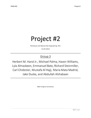
  • 16. PNGE 441 Project2 16 | P a g e Figure 8: Each sub-scenario's calculated NPV at a 18% interest rate from Jan 1st 2014 - Jan 1st 2024 The following questions are answered below (see figure 9): C) What is the best scenario if we plan to produce until 1/1/2024? D) What is the best scenario if we plan to produce until 1/1/2023? E) What is the best scenario if we plan to produce until 1/1/2022? F) What is the best scenario if we plan to produce until 1/1/2021? G) What is the best scenario if we plan to produce until 1/1/2020? Year Scen. 1 Scen. 2 Scen. 3 Scen. 4 Scen. 5 Scen. 6 Scen. 7 Scen. 8 Scen. 9 Scen. 10 2014 -115000000 -140000000 -165000000 -215000000 -275000000 -130000000 -155000000 -180000000 -230000000 -290000000 2015 320023580.7 370740884.1 405611020.3 458714303.5 487744662.8 296223296.3 347346040.7 382980003.6 439674293.7 464249927.8 2016 644640325.2 738001411.9 805773509.9 910069898.8 980221621 613938539.9 707587367 777705796.5 889008742 953815310.1 2017 902809910.7 1020471922 1106423935 1236992705 1325336648 867952217.4 985845147.7 1075391369 1216050048 1300610083 2018 1111555360 1240482068 1333365405 1470749691 1557161433 1074302686 1202973451 1300905401 1451020158 1535734681 2019 1280352357 1409116312 1498428432 1624868389 1693051010 1241960183 1370070909 1466354008 1607386297 1676448301 2020 1414862775 1533544245 1610266746 1710943696 1749703805 1376698460 1494726525 1580547012 1696806509 1738670111 2021 1519956243 1620332072 1677926674 1744113360 1746565419 1483419090 1583725731 1652110418 1734011950 1741113517 2022 1598074057 1673739877 1708383180 1736540706 1700690556 1564463343 1641049103 1687369794 1731421408 1700144062 2023 1652124853 1698853846 1708943834 1698931461 1622910674 1622530422 1671337217 1693123040 1699059981 1627702450 2024 1683665965 1700201695 1686072604 1638357737 1521004222 1658952955 1678619901 1675362341 1643799465 1531032382 2% Interest Rate NPV Figure 9: The best case scenarios according to the year and interest rate. This is a crucial step to determining the most feasible scenario for your project. Figure 10: 2% interest rate NPV calculated for each scenario for each year. Interest 2020 2021 2022 2023 2024 2% 5 4 3 2 1 6% 5 4 3 2 7 10% 5 4 3 2 7 14% 5 4 3 2 7 18% 5 4 3 2 7 Best Scenario
  • 17. PNGE 441 Project2 17 | P a g e Year Scen.1 Scen.2 Scen.3 Scen.4 Scen.5 Scen.6 Scen.7 Scen.8 Scen.9 Scen.10 2014 -115000000 -140000000 -165000000 -215000000 -275000000 -130000000 -155000000 -180000000 -230000000 -290000000 2015 303607596.5 351467643.2 384078529 433291122.2 458961845.4 280139398.3 328389586.4 361735475.2 414403565.6 435787666.4 2016 604187216.4 691533372.2 754609905 851224872.1 914972015.6 574328557.7 661955869.6 727232729.5 830465829.8 889101856.2 2017 834219079.6 943217619.5 1022492651 1142516591 1222473197 800657462.3 909886529.6 992473759.9 1121863133 1198099710 2018 1013194851 1131851602 1217069466 1342936945 1421236906 977579806.3 1096049657 1185826707 1323323605 1399692637 2019 1152458012 1270980487 1353251976 1470090019 1533350346 1115902842 1233910641 1322327335 1452330893 1515786074 2020 1259245842 1369763831 1442040422 1538425211 1578327004 1222871569 1332874743 1412985168 1523321605 1565183973 2021 1339531112 1436064660 1493728654 1563764896 1575929461 1304399895 1400864936 1467655429 1551744388 1567050593 2022 1396956578 1475325463 1516117645 1558198135 1542206226 1363976627 1443004126 1493575076 1549840045 1536933389 2023 1435190676 1493090419 1516514237 1531594353 1487186802 1405051738 1464429134 1497644769 1526948431 1485690116 2024 1456660084 1494007873 1500946245 1490363024 1417821106 1429843832 1469386312 1485555414 1489333696 1419888723 6% Interest Rate NPV Year Scen. 1 Scen. 2 Scen. 3 Scen. 4 Scen. 5 Scen. 6 Scen. 7 Scen. 8 Scen. 9 Scen. 10 2014 -115000000 -140000000 -165000000 -215000000 -275000000 -130000000 -155000000 -180000000 -230000000 -290000000 2015 274231624.8 316978685.8 345546702.4 387797008.4 407455751 251357686.1 294467510.1 323718950.6 369182262.8 384855198.5 2016 534104863.5 610990576.4 665898390.7 749131543.2 801710157.9 505705900.6 582860150.8 639718269.6 728898760.2 776778731.7 2017 719027909.7 813320014.8 881249832.7 983301502.1 1048910935 687652131.5 782172073.4 852946031.3 963153598.5 1025182686 2018 852810099 954321598.2 1026693610 1133113253 1197484364 819899408.9 921326722.6 997474982.8 1113742825 1175870921 2019 949602512.2 1051020685 1121344871 1221488763 1275406841 916038404.5 1017144578 1092347346 1203407074 1256559625 2020 1018615026 1114860234 1178725135 1265650943 1304473376 985167824.3 1081100943 1150935716 1249285406 1288483423 2021 1066858988 1154700851 1209784943 1280877732 1303032676 1034158748 1121956710 1183787446 1266364848 1289605088 2022 1098944771 1176637349 1222294520 1277767372 1284190227 1067446524 1145501472 1198269735 1265300820 1272777465 2023 1118808463 1185866744 1222500561 1263945957 1255606085 1088786202 1156632367 1200384055 1253407981 1246155140 2024 1129179691 1186309939 1214980130 1244028335 1222097592 1100762521 1159027032 1194544049 1235237428 1214368456 14% Interest Rate NPV Year Scen.1 Scen.2 Scen.3 Scen.4 Scen.5 Scen.6 Scen.7 Scen.8 Scen.9 Scen.10 2014 -115000000 -140000000 -165000000 -215000000 -275000000 -130000000 -155000000 -180000000 -230000000 -290000000 2015 261037332.5 301487882.8 328240034.5 367363211.5 384321657.7 238430306.9 279231323.3 306643732 348870999.6 361978751.1 2016 503590665.5 575904611.6 627241078.8 704615697.4 752299988.1 475826844.9 548403311.2 601582481.5 684613286.4 727781554.7 2017 670338257.5 758347781 821426363.6 915769891.4 975204245.3 639890202.6 728125546 793852815.3 895844017.2 951770732.9 2018 786882191.8 881180867.8 948129253.7 1046277928 1104633522 755097003.3 849349681.9 919758757.7 1027029349 1083042316 2019 868344279.9 962564410.8 1027789313 1120656212 1170214361 836009164.3 929991565.9 999604899.9 1102492257 1150951257 2020 924457463.5 1014471524 1074444464 1156563910 1193847985 892217402.9 981993660.4 1047242347 1139795336 1176908086 2021 962354292.8 1045767317 1098842715 1168524930 1192716279 930700988.9 1014086879 1073048196 1153211662 1177789181 2022 986704092.5 1062414856 1108336193 1166164488 1178416805 955962977.6 1031954925 1084038760 1152404174 1165018751 2023 1001267586 1069181586 1108487256 1156031020 1157459725 971608622.3 1040115781 1085588919 1143684683 1145500020 2024 1008613717 1069495509 1103160398 1141923005 1133725048 980091667.7 1041811965 1081452337 1130814149 1122984931 18% Interest Rate NPV Figure 11: 6% interest rate NPV calculated for each scenario for each year. Year Scen. 1 Scen. 2 Scen. 3 Scen. 4 Scen. 5 Scen. 6 Scen. 7 Scen. 8 Scen. 9 Scen. 10 2014 -115000000 -140000000 -165000000 -215000000 -275000000 -130000000 -155000000 -180000000 -230000000 -290000000 2015 288385502.1 333596092.5 364112037 409716899.6 432272323.7 265225238.3 310811783.2 342036003.4 390970708.7 409395387.6 2016 567502246.7 649379442.2 708185635.5 797808107.4 855721106.6 538407833 620559779.8 681434941.3 777324064.1 830340696.5 2017 773341187 874593541 947894603.8 1058464079 1130881758 740933262.5 842415063.8 918780028.5 1038074515 1106840612 2018 927669981.4 1037250502 1115676002 1231284295 1302273468 893491409.4 1002941434 1085506100 1211791614 1280671926 2019 1043388309 1152857255 1228834516 1336939954 1395432203 1008428556 1117494647 1198928948 1318988000 1377137769 2020 1128895146 1231954764 1299928939 1391657109 1431445780 1094080241 1196736892 1271520221 1375831474 1416691510 2021 1190843266 1283112489 1339811583 1411209211 1429595835 1156987503 1249198130 1313703799 1397762496 1418131794 2022 1233541506 1312304541 1356458736 1407070092 1404521197 1201285299 1280530383 1332976142 1396346537 1395738392 2023 1260936390 1325033202 1356742895 1388008375 1365099560 1230715780 1295881487 1335892094 1379944604 1359022381 2024 1275759928 1325666658 1345993986 1359540232 1317206063 1247833465 1299304167 1327545007 1353973536 1313589855 10% Interest Rate NPV Figure 12: 10% interest rate NPV calculated for each scenario for each year. Figure 13: 14% interest rate NPV calculated for each scenario for each year. Figure 14: 18% interest rate NPV calculated for each scenario for each year.
  • 18. PNGE 441 Project2 18 | P a g e When selecting the best case scenario for each year at each interest rate, the net present value (NPV) was taken into account. Along with the highest magnitude NPV value, the slope of each line is investigated to determine the best case scenario. The scenario with the highest NPV value and still increasing slope is chosen as the best case scenario for each year and interest rate. If the slope is decreasing at any time selected, the value of the scenario is already decreasing and is therefore losing money. When the slope is increasing, the scenario is still increasing in value and is still an operable scenario. As soon as the slope begins its decline, the scenario is not feasible. The best case scenarios for each year and interest rate can be found in the table above. While adding more wells increases recovery factors initially, there is a steep drop off as time passes. Adding more wells will increase profits in the early stages of production, but will increase costs later in production. This also pertains to injection wells. As more injection wells are added, the production rates will increase and recovery factors will be high. But, as time passes, the recovery factor declines rapidly, and costs will start to overcome profit from production. Therefore, it is financially smarter to produce with fewer wells. The oil and gas recovery factors for each scenario vs. time and the oil and gas recovery factors vs. NPV for each interest rate can be found in the charts below. Figure 15: Oil recovery factor vs. time 0% 5% 10% 15% 20% 25% 30% 2012 2014 2016 2018 2020 2022 2024 2026 OilRF(%) Time (years) Oil Recovery Factor vs. Time Scenario 1 Scenario 2 Scenario 3 Scenario 4 Scenario 5 Scenario 6 Scenario 7 Scenario 8 Scenario 9 Scenario 10
  • 19. PNGE 441 Project2 19 | P a g e Figure 16: Gas recovery factor vs. time 0% 5% 10% 15% 20% 25% 30% 35% 40% 45% 2012 2014 2016 2018 2020 2022 2024 2026 GasRF(%) Time (years) Gas Recovery Factor vs. Time Scenario 1 Scenario 2 Scenario 3 Scenario 4 Scenario 5 Scenario 6 Scenario 7 Scenario 8 Scenario 9 Scenario 10
  • 20. PNGE 441 Project2 20 | P a g e Figure 17: Oil RF vs. NPV at 2% interest -5E+08 0 500000000 1E+09 1.5E+09 2E+09 15% 17% 19% 21% 23% 25% 27% 29% NPV Oil RF 2% Interest Rate Scenario 1 Scenario 2 Scenario 3 Scenario 4 Scenario 5 Scenario 6 Scenario 7 Scenario 8 Scenario 9 Scenario 10
  • 21. PNGE 441 Project2 21 | P a g e Figure 18: Gas RF vs. NPV at 2% interest -5E+08 0 500000000 1E+09 1.5E+09 2E+09 15% 20% 25% 30% 35% 40% 45% NPV Gas RF 2% Interest Rate Scenario 1 Scenario 2 Scenario 3 Scenario 4 Scenario 5 Scenario 6 Scenario 7 Scenario 8 Scenario 9 Scenario 10
  • 22. PNGE 441 Project2 22 | P a g e
  • 23. PNGE 441 Project2 23 | P a g e Figure 19: Oil RF vs. NPV at 6% interest -5E+08 0 500000000 1E+09 1.5E+09 2E+09 15% 17% 19% 21% 23% 25% 27% 29% NPV Oil RF 6% Interest Rate Scenario 1 Scenario 2 Scenario 3 Scenario 4 Scenario 5 Scenario 6 Scenario 7 Scenario 8 Scenario 9 Scenario 10
  • 24. PNGE 441 Project2 24 | P a g e Figure 20: Gas RF vs. NPV at 6% interest -5E+08 0 500000000 1E+09 1.5E+09 2E+09 15% 20% 25% 30% 35% 40% 45% NPV Gas RF 6% Interest Rate Scenario 1 Scenario 2 Scenario 3 Scenario 4 Scenario 5 Scenario 6 Scenario 7 Scenario 8 Scenario 9 Scenario 10
  • 25. PNGE 441 Project2 25 | P a g e Figure 21: Oil RF vs. NPV at 10% -4E+08 -2E+08 0 200000000 400000000 600000000 800000000 1E+09 1.2E+09 1.4E+09 1.6E+09 15% 17% 19% 21% 23% 25% 27% 29% NPV Oil RF 10% Interest Rate Scenario 1 Scenario 2 Scenario 3 Scenario 4 Scenario 5 Scenario 6 Scenario 7 Scenario 8 Scenario 9 Scenario 10
  • 26. PNGE 441 Project2 26 | P a g e Figure 22: Gas RF vs. NPV at 10% interest -4E+08 -2E+08 0 200000000 400000000 600000000 800000000 1E+09 1.2E+09 1.4E+09 1.6E+09 15% 20% 25% 30% 35% 40% 45% NPV Gas RF 10% Interest Rate Scenario 1 Scenario 2 Scenario 3 Scenario 4 Scenario 5 Scenario 6 Scenario 7 Scenario 8 Scenario 9 Scenario 10
  • 27. PNGE 441 Project2 27 | P a g e Figure 23: Oil RF vs. NPV at 14% interest -4E+08 -2E+08 0 200000000 400000000 600000000 800000000 1E+09 1.2E+09 1.4E+09 15% 17% 19% 21% 23% 25% 27% 29% NPV Oil RF 14% Interest Rate Scenario 1 Scenario 2 Scenario 3 Scenario 4 Scenario 5 Scenario 6 Scenario 7 Scenario 8 Scenario 9 Scenario 10
  • 28. PNGE 441 Project2 28 | P a g e Figure 24: Gas RF vs. NPV at 14% interest -4E+08 -2E+08 0 200000000 400000000 600000000 800000000 1E+09 1.2E+09 1.4E+09 15% 20% 25% 30% 35% 40% 45% NPV Gas RF 14% Interest Rate Scenario 1 Scenario 2 Scenario 3 Scenario 4 Scenario 5 Scenario 6 Scenario 7 Scenario 8 Scenario 9 Scenario 10
  • 29. PNGE 441 Project2 29 | P a g e Figure 25: Oil RF vs. NPV at 18% interest -4E+08 -2E+08 0 200000000 400000000 600000000 800000000 1E+09 1.2E+09 1.4E+09 15% 17% 19% 21% 23% 25% 27% 29% NPV Oil RF 18% Interest Rate Scenario 1 Scenario 2 Scenario 3 Scenario 4 Scenario 5 Scenario 6 Scenario 7 Scenario 8 Scenario 9 Scenario 10
  • 30. PNGE 441 Project2 30 | P a g e Figure 26: Gas RF vs. NPV at 18% interest rate The following is our Present Value Profile (PVP). The PVP is a plot of each scenario’s NPV versus interest rate at the final simulation year of 2024. This plot gives the Internal Rate of Return (IRR), which tells when each scenario becomes unprofitable. -4E+08 -2E+08 0 200000000 400000000 600000000 800000000 1E+09 1.2E+09 1.4E+09 15% 20% 25% 30% 35% 40% 45% NPV Gas RF 18% Interest Rate Scenario 1 Scenario 2 Scenario 3 Scenario 4 Scenario 5 Scenario 6 Scenario 7 Scenario 8 Scenario 9 Scenario 10
  • 31. PNGE 441 Project2 31 | P a g e Figure 27: PVP for 2024
  • 32. PNGE 441 Project2 32 | P a g e Figure 28: PVP at 2024 (zoomed-in for clarity). IRR values are visible.
  • 33. PNGE 441 Project2 33 | P a g e Figure 29: PVP at 2024 (zoomed-in at the top).
  • 34. PNGE 441 Project2 34 | P a g e The Internal Rate of Return (IRR) is calculated and the results are shown below in figure 19. Scenario IRR (%) 1 362.8310009850% 2 346.3247526200% 3 325.1308833650% 4 288.8635597640% 5 249.6317477300% 6 311.5347783000% 7 304.7727526830% 8 291.5265525600% 9 266.4301287065% 10 232.4751121408% Figure 30: IRR values for each scenario at 1/1/2024
  • 35. PNGE 441 Project2 35 | P a g e Conclusions To conclude, In order to go forward with the project, two important questions must be addressed: What is the interest rate? And, how long will you plan to produce? The answers to these questions must be taken into account, and figure 9 is used to find the most profitable scenario. For example, if the interest rate happens to be 14% and the decision to produce until 2022 is made, the best scenario to put into place will be scenario 2. Scenario 3 suggests that 6 injection wells are to be drilled along with 22 additional producing wells. This scenario yields the highest NPV while maintaining a positive slope at 2022. However, there are scenarios with higher NPV values, but are in fact decreasing with respect to time. So, it is important to pick a scenario that has a positive slope (NPV vs. time) or you end up losing money. Once a scenario has a negative slope, it should be shut down because it is not profitable anymore. Other factors that affect your decision of scenarios is the number of well, which translates into direct costs. The more wells that are drilled will yield higher operational costs and unplanned maintenance costs. So, to pick the correct scenario for your project, a proper cost analysis should be made. Also, the internal rate of return (IRR) will ultimately help you decide on a scenario. For example (as shown in figures 27 – 30), if the decision to produce until January 1st, 2024 is made, the scenario with the highest rate of return after 10 years of water-flooding will be scenario 1 (362.83%) (Refer to figure 30). Additionally, the graphs of the oil and gas recovery factor vs. NPV help support your decision. Although scenario’s 5 and 10 have the highest NPV values in the plot, they also have the highest amount of wells drilled. This transmits to higher operational costs, which will have negative effects on profit. Now, taking a cost analysis in consideration, scenario one has the least amount of wells drilled in both cases. And the IRR for scenario 1 is the highest (362.83%). Conversely, scenario 7 has an IRR of 304.77%. Since scenario 1 has an IRR that is significantly higher, this is considered the most desirable project to undertake. So, analytically, this makes sense. It turns out that the IRR, in this project, relates to the cost analysis at 2024. Essentially, the least amount of wells yields the least amount of cost, which, in turn, delivers the highest IRR. Scenario 1 demonstrates this conclusion, and it is the best decision if you plan to produce until or beyond 2024. Figure 31: Finalized Best Scenarios after taking in account the Internal Rate of Return. Initially scenario 7 is the best scenario in 2024 when just considering NPV vs. time, but the IRR is significantlylower than scenario 1. Therefore, scenario 1 is the best scenario in 2024. in 2024 1 Best Scenario After Considering IRR
  • 36. PNGE 441 Project2 36 | P a g e References Zamirian, Mehrdad. PNGE441 Class Notes. “Economic Analysis-Investment Decisions” Lecture. Fall 2014. Zamirian, Mehrdad. PNGE 441 Class Notes. “Economic Analysis – Basic Concepts” Lecture. Fall 2014. Zamirian, Mehrdad. PNGE 441 Class Notes. “Economic Analysis - Interest Rates” Lecture. Fall 2014. Hand, Herbert. PNGE 441 Project 1 Report. “PNGE441_Fall2014_Hand_Herbert_Project1” Report. Fall 2014