This document provides definitions and formulas for calculating curl, divergence, and line integrals. It defines curl as the measure of rotation in a vector field and divergence as the measure of how a vector field spreads out from a point. Formulas are given for calculating curl, divergence, and line integrals over curves with respect to arc length, x, y, and vector fields. It also discusses properties of conservative and irrotational vector fields as they relate to these calculations.

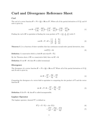
1. Curl and Divergence Reference Sheet
Curl
The curl of a vector function F = Pi + Qj + Rk on R3
, Where all of the partial derivatives of P, Q, and R
exist is given by
curl F =
∂R
∂y
−
∂Q
∂z
i +
∂P
∂z
−
∂R
∂x
j +
∂Q
∂x
−
∂P
∂y
k (1)
Finding the curl of F is equivalent of finding the cross product of = ∂
∂x , ∂
∂y , ∂
∂z with F:
curl F = × F =
i j k
∂
∂x
∂
∂y
∂
∂z
P Q R
(2)
Theorem If f is a function of three variables that has continuous second-order partial derivatives, then
curl( f) = 0. (3)
Definition A conservative field is a field F such that F = f.
By the Theorem above, if F is a conservative field, then curl F = 0.
Definition If curl F = 0, then F is called irrotational.
Divergence
The divergence of a vector function F = Pi + Qj + Rk on R3
Where all of the partial derivatives of P, Q,
and R exist is given by
div F =
∂P
∂x
+
∂Q
∂y
+
∂R
∂z
(4)
Computing the divergence of a vector field is equivalent to computing the dot product of and the vector
function F:
div F = · F =
∂P
∂x
+
∂Q
∂y
+
∂R
∂z
(5)
Definition If div F = 0, then F is called incompressible.
Laplace Operator
The Laplace operator, denoted 2
, is defined as
2
f = · f = div ( f) (6)
=
∂2
P
∂x2
+
∂2
Q
∂y2
+
∂2
R
∂y2
(7)
1

2. Line Integrals
Line Integrals with Respect to Arc Length
If we have a curve defined in the xy−plane by the parametric equations x = x(t), y = y(t) for a ≤ t ≤ b,
then the following formula can be used to evaluate the line integral:
C
f(x, y)ds =
b
a
f(x(t), y(t))
dx
dt
2
+
dy
dt
2
dt (8)
Piecewise-Smooth Curves
Suppose that C is a piecewise-smooth curve (C is the union of a finite number of smooth curves, C1, C2, . . . , Cn,
then the line integral of f over C is given by the sum of the line integral over each of the pieces:
C
= f(x, y)ds =
C
f(x, y)ds + · · · +
Cn
f(x, y)ds (9)
To compute a line integral with respect to arc-length:
In the case that C is a piecewise-smooth curve, repeat steps 1-4 for each smooth piece, then sum the values.
1. Parameterize f(x, y) (find parametric equations x = x(t), y = y(t)).
2. Find ds = dx
dt
2
+ dy
dt
2
dt.
3. Plug in parametric equations and ds to obtain
b
a
f(x(t), y(t)) dx
dt
2
+ dy
dt
2
dt.
4. Evaluate the integral.
Line Integrals with Respect to x and/or y
To compute the line integrals with respect to x and y, we again find parametric equations x = x(t), y = y(t)
and their derivatives with respect to t: dx = x (t), dy = y (t). Then
C
f(x, y)dx =
b
a
f(x(t), y(t))x (t)dt,
C
f(x, y)dy =
b
a
f(x(t), y(t))y (t)dt (10)
Line integrals with respect to x and y often happen together. In this case, we usually write
C
P(x, y)dx +
C
Q(x, y)dy =
C
P(x, y)dx + Q(x, y)dy (11)
For line integrals in space, the above formulas can easily be generalized to three variables:
C
f(x, y, z)ds =
b
a
f(x(t), y(t), z(t))
dx
dt
2
+
dy
dt
2
+
dz
dt
2
dt (12)
2

3. and
C
P(x, y, z)dx + Q(x, y, z)dy + R(x, y, z)dz (13)
Line Integrals of Vector Fields
Let F be a continuous vector field defined on a smooth curve C given by a vector function r(t), a ≤ t ≤ b.
Then the line integral of F along C is defined to be
C
F · dr = F(r(t)) · r (t)dt =
C
F · Tds (14)
where r(t) = (x(t), y(t), z(t)) and dr = r (t)dt. Using this formula, we can compute the work, W, done
by the force field F. So essentially, the work done is the line integral with respect to the arc length of the
tangential component of the force. For good measure,
W =
C
F · Tds (15)
Finally, we make the connection between line integrals of vector fields and line integrals of scalar fields. for
F = Pi + Qj + Rk,
C
F · dr =
C
Pdx + Qdy + Rdz (16)
The Fundamental Theorem for Line Integrals
let F = f be a conservative vector field. It turns out that for such a field, the line integral over a curve
C depends only on the endpoints of C. So if C is a smooth curve given by r(t), a ≤ t ≤ b, and f is a
differentiable function of two or three variables in which f is continuous on C, then
C
f · dr = f(r(b)) − f(r(a)). (17)
So basically, if we have two piecewise-smooth curves, C1 and C2, with the same initial and terminal points,
then the above formula tells us that
C1
f · dr =
C2
f · dr (18)
To reiterate, the line integral of a conservative vector field F with domain D depends only on
the initial point and the terminal point of a curve.
Definition A curve is called closed if its terminal point coincides with its initial point, i.e. r(a) = r(b).
Theorem C
F · dr is independent of path in D (the domain of F) if and only if C
F · dr = 0 for every
closed path C in D.
Theorem If C
F · dr is independent of path in D, then F is a conservative vector field on D.
Theorem If F(x, y) = P(x, y)i + Q(x, y)j is a conservative vector field, where P and Q have continuous
first-order partial derivatives on a domain D then throughout D we have
∂P
∂y
=
∂Q
∂x
(19)
Theorem Let F = Pi + Qj be a vector field on an open, simply-connected region D. Suppose that P and
Q have continuous first-order derivatives and ∂P
∂y = ∂Q
∂x throughout D. Then F is conservative.
3