1. Testing Milne-Eddington Inversion Codes Against One-Dimensional Model Atmospheres
Erica Lastufka1, Sarah Jaeggli1, Charles Kankelborg1, & Han Uitenbroek2
1
Department of Physics, Montana State University, 2
National Solar Observatory, Sacramento Peak
Abstract
Properties of solar vector magnetic fields can be determined by the inversion of polarization
spectra. It is therefore important to have accurate inversion methods. Milne-Eddington inversions,
used almost exclusively in the photosphere, assume a thin, flat atmosphere and are one of the
most widely used inversion techniques. To investigate the potential weaknesses of parameterizing
a stratified atmosphere using a single set of properties, we examine the consequences of using a
Milne-Eddington inversion to invert spectra of complex atmospheres. Han Uitenbroek’s Rybicki-
Hummer radiative transfer and chemical equilibrium code was used to generate a series of one-
dimensional model atmospheres with predetermined magnetic field configurations, with strengths
up 3000 G and inclination and azimuthal angles from 0 to 180 degrees. We examined the Stokes
profiles of the Fe 15648.5 line, which with a Land´e g-factor of 3.0 is very sensitive to the magnetic
field. Using a simple Milne-Eddington inversion code, we examined the ranges in which the code
accurately parameterized the magnetic field. To investigate the confidence intervals associated
with the inverted parameters, we used the BayesME code developed by Andres Asensio Ramos.
We discuss the key assumptions and limitations of a Milne-Eddington inversion.
1.Milne-Eddington Inversions
A Milne-Eddington inversion is based on treating the source function as linear with optical depth,
as it would be in a thin, flat atmosphere. In such a region, line formation occurs at a single height,
absorption is constant, and local thermodynamic equilibrium is a valid assumption. This makes it
simple to calculate the properties of the atmosphere and magnetic field that result in fits to Stokes
I, Q, U, and V spectral line profiles.
We chose magnetically sensitive iron lines to analyze the accuracy of the Milne-Eddington
inversion technique. The common diagnostic infrared lines at 15645,15648.5 and 15652.8
angstroms have Land´e factors of 1.9, 3.0, and 1.5 respectively.
Figure 1: Intensity of Fe I 15645,15648.5 and 15652.8 at different effective temperatures
2.Atmospheric Models
We used a series of complex model atmospheres to test the accuracy of our Milne-Eddington
inversion. Each atmosphere consisted of temperature, electron density, velocity, and hydrogen
ionization population data for a column approximately 0.1 Mm deep. The atmospheres, with
characteristic temperatures within 1000 K of the quiet Sun temperature, were used together
with one-dimensional magnetic fields of varying magnitude, inclination and azimuth. To
simultaneously solve the radiative transfer and statistical equilibrium problems under non-LTE
conditions, we used Han Uitenbroek’s Rybicki-Hummer radiative transfer code. This generated
synthetic Stokes profiles. The table lists the properties of the atmosphere, magnetic field, and
spectral line used in the inversion of the profiles.
Parameter Physical meaning Typical range
B0 Source function 0 ≤ B0 ≤ 1 pixels
B1 Gradient of source function 0 ≤ B1 ≤ 1 pixels
B Field strength 100 ≤ B1 ≤ 3000 G
lc Line center 15648.5 ˚A
dw Doppler width 0.13 pixels
r0 Inclination angle 0 ≤ r0 ≤ 90 degrees
ρ0 Azimuthal angle 0 ≤ ρ0 ≤ 180 degrees
η0 Line-to-continuum absorption ration 10
a Damping parameter 10 nm
3. Inversion Codes
To invert the synthetic spectra, we used two simple Milne-Eddington inversion codes. The first,
named the Two-Component Magneto-Optical code (2cmo), was developed in Jaeggli (2011). It
uses chi-squared curve fitting to Faraday-Voigt profiles to quickly invert Stokes profiles. 2cmo can
fit multiple lines simultaneously in order to better constrain the solution.
Most Milne-Eddington inversion codes are unable to provide statistical information about
confidence intervals. Using a Bayesian approach to the inversion such as in Asensino Ramos
(2007) makes this possible. Bayes ME uses the error associated with each wavelength point to
determine the confidence intervals. We used a photon noise distribution to estimate error. The
Markov Chain Monte Carlo used in calculation requires much more CPU time than 2cmo, so
although BayesME is also capable of fitting more than one line profile at a time, we opted to use a
reduced wavelength range centered on Fe I 15648. Figure 3 demonstrates the fits to the profiles of
the different codes.
It is clear that small signals in Stokes Q, U and V may be lost among the noise.
Figure 2: 2cmo and BayesME fits to the RH-generated Stokes spectra with the addition of
Poissonian noise.
4. Results
Figures 4 and 5 show how the values obtained from the inversion compare to the known magnetic
field properties.The magnetic field strength is divided into two categories, high (≥ 1000 G) and
low (≤ 500 G). These colour coding in these plots is according to the characteristic temperature
of the atmosphere. The plots demonstrating the results of the angular inversions are colour coded
according to the strength of the magnetic field.
Figure 3: 2cmo inversion: inverted parameter values vs. actual values
From figure 4, showing the inverted parameters obtained by 2cmo, the following are evident:
• For low magnetic field strengths, inversion is far less accurate than for high field strengths
• For high field strengths, inversion accuracy improves with higher atmospheric temperatures
• Inversion of angular parameters improve as field strength increases
• Azimuthal angle is determined much more poorly than inclination angle
Addition of Poissonian noise to the profiles before using the 2cmo inversion led to similar results
in terms of the magnetic field strength. However, the angular parameters were at times very
erroneous, since small signals in Q and U, resulting from specific angular configurations or at
low magnetic field strengths, led to an inability to distinguish Stokes Q and U from the noise.
Trends in the BayesMe inversion data resemble those listed previously for the 2cmo data. To
better understand the significance of the confidence intervals calculated by BayesME, Figure 5
presents a histogram of the one-sigma errors associated with the inverted parameter. We follow
the colour coding of Figure 4, and similarly include a plot of the residuals, this time only for
selected atmospheric temperatures and field strengths. Confidence intervals are represented with
error bars; in most cases they are quite small. The primary results are listed below.
Figure 4: Confidence intervals obtained with BayesME and their frequency for inverted parameters
• Small one-sigma confidence intervals do not always mean a more accurate inversion. For
example, for residuals greater than 100 G, confidence internals were between 10 and 15 G.
• The confidence intervals were on the order of magnitude of the residuals 93% of the time for
high B, 2% for low B, 28% for inclination angle, and 9% for azimuthal angle.
• 90% of the one-sigma errors were within two orders of magnitude of the residuals, with the
majority of outliers coming from low B field inversions.
5. Conclusions
Milne-Eddington inversions of one-dimensional atmospheres are very well suited to regions with
magnetic field strengths greater than 1000 G with temperatures near or above the quiet Sun
temperature. This is due to the formation height and amount of Zeeman splitting of our chosen
g=3 Fe I line. Noise of any sort significantly reduces the accuracy of the inversions, especially in
calculating the angular parameters which depend on Stokes Q and V. The assumption of a thin,
flat atmosphere in LTE made by the Milne Eddington approximation can be very accurate in the
photosphere. When choosing to use an inversion of this sort, one must be aware of the limitations
of this simplistic assumption in describing a complex atmosphere.
6. References
Asensino Ramos, A., Mart´ıinez Gonz´alez, M.J. and Rubi˜no-Mart´ın, J.A. 2007, A& A, 476
Jaeggli, S. A. 2011. PhD thesis. Univ. of Hawai’i
Contact
Erica Lastufka email: elastufka@physics.montana.edu
Graduate Student address: Montana State University
Department of Physics
Bozeman, Mt 59715
phone: 713.534.2224