The document contains examples of functions of several variables and their domains and ranges. It provides equations for various functions and graphs their surfaces over different domains. Some key examples include functions defined by equations like x2 + y2 = 1, 2, 3 and functions where increasing one variable by a fixed amount increases the output by a fixed amount.

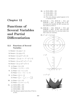
1. 12. (a) R(150, 2000) = 333
(b) R(160, 2000) = 354
(c) R(170, 2000) = 375
(d) The extra distance gained appears to be
a constant 21 feet.
Chapter 12 13. H(80, 20) = 77.4, H(80, 40) = 80.4, and
H(80, 60) = 82.8. It appears that at 80◦ ,
increasing the humidity by 20% increases the
heat index by about 3.
Functions of 14. H(90, 20) = 86.5, H(90, 40) = 92.3, and
H(90, 60) = 100.5. At 90◦ , each extra 20%
Several Variables humidity adds about 7 to the heat index (but
this is also not constant).
and Partial 15. x2 + y 2 = 1 or 2 or 3
Differentiation 1.5
1.0
z=3
z=2
z=1
0.5
0.0
12.1 Functions of Several −1.5 −1.0
x
−0.5 0.0 0.5 1.0 1.5
−0.5
Variables y
−1.0
1. Domain = {(x, y)|y = −x}
−1.5
2
2. Domain = {(x, y)|y = x }
z = y2
3. Domain = (x, y)| x2 + y 2 ≥ 1
2.0
4. Domain = (x, y) | 1 < x2 + y 2 ≤ 4
1.5
5. Domain = {(x, y, z)|x2 + y 2 + z 2 < 4}
z 1.0
6. Domain = {(x, y, z)|x2 + y 2 = z}
0.5
7. (a) Range = {z|z ≥ 0}
(b) Range = { z | 0 ≤ z ≤ 2 } 0.0
−1.0 −0.5 0.0 0.5 1.0
8. (a) Range = {z| − 1 ≤ z ≤ 1} y
(b) Range = { z | − 1 ≤ z ≤ 1 }
9. (a) Range = {z|z ≥ −1} z = x2 + y 2
π π
(b) Range = z | − ≤ z <
4 2 8
10. (a) Range = {z|z > 0} 6
(b) Range = z | 0 < z ≤ e2
4
11. (a) R(150, 1000) = 312
2
(b) R(150, 2000) = 333
0
(c) R(150, 3000) = 350 2 1 1 00 −1 −2
−1 −2
2 y
x
(d) The distance gained varies from 17 feet to
21 feet.
660

2. 12.1. FUNCTIONS OF SEVERAL VARIABLES 661
16. For x = 0, z = −y 2 3
2
y
−1.0 −0.5 0.0 0.5 1.0 z=3
0.0 1 z=2
z=1
−0.5 0
−3 −2 −1 0 1 2 3
x
−1
z −1.0
y
−2
−1.5
−3
−2.0
x = 0 ⇒ z = |y|
For y = 0, z = x2 5
2.0
4
1.5
3
z
z 1.0 2
1
0.5
0
0.0 −5.0 −2.5 0.0 2.5 5.0
−1.0 −0.5 0.0 0.5 1.0 y
x
z= x2 + y 2
z = x2 − y 2
10
8 5
6
4
4
3
2
2
−5.0 0
−2.5 −5.0
−2.5 1
y 0.0
0.0
2.5 −2
2.5 x
5.0
5.0 0 4
−4 −4 −2 2
00
−2 2 4
x
−4
−6 y
−8
−10
x2 − y 2 = 1 or − 1. For z = −1; z = 1. 18. 2x2 − y = 0 or 1 or 2
10
8
8
7
6
6
4
5
2
4
0
3
−10 −8 −6 −4 −2 0 2 4 6 8 10 2.7
−2
x 2
.7
−4
1
y
−6
0 1.7
−8 −2 −1 0 1 2
−1
x
−10
−2
17. x2 + y 2 = 1 or 2 or 3 z = −y

3. 662 CHAPTER 12. FUNCTIONS OF SEVERAL VARS. AND PARTIAL DIFF.
5 2.0
4 1.6
3 1.2
2 0.8
1 0.4
0 0.0
−5 −4 −3 −2 −1 0 1 2 3 4 5 −2 −1 0 1 2
−1 −0.4
y x
−2 −0.8
z y
−3 −1.2
−4 −1.6
−5 −2.0
z = 2x2 − y z= 4 − x2 − y 2
10.0
2.0
7.5
1.5
5.0
1.0
2.5 4 0.5
2 4
−4
−4 0
0.0
−2 0.0 2
−2
y −2
x 0 x 00
2
−4 4 −2 2
−2.5
y 4
−4
19. z = 4 − y2 20. z = 0 or y 2 − x2 = 4
5 10
4
8
3
6
2 4
1
2
0
0
−5 −4 −3 −2 −1 0 1 2 3 4 5
−1 −10 −8 −6 −4 −2 0 2 4 6 8 10
y −2
x
−2
−4
z
y
−3
−6
−4
−8
−5
−10
√
z= 4 − x2 z= 5 − y 2 . For x =1 or -1
5.0
2.5
2
z
1
0.0
−5 −4 −3 −2 −1 0 1 2 3 4 5
x
0
z −2.5 −2 −1 0 1 2
y
−5.0
4 − x2 − y 2 = 0 or 1 z= 4 − y2

4. 12.1. FUNCTIONS OF SEVERAL VARIABLES 663
2 2
z 1 1
0 4 3 0
2 1 1 2 3
−2 −1 0
0
−2 −1 0 1 2 y −1 −2
−3 x
y
−1
z= 4 + x2 − y 2
2.0
2.2
4
1.5
2.1 1.0
2 3
y
0.5 2
2.0 1
0.0
0 x
0
−1
−0.5
1.9 −2
−1.0 −2
1.8
1.0 1.0
0.5 0.5
0.0
−0.5 −0.5
−1.0 −1.0
x y
22. (a)
21. (a)
2.0
3
x 2
1.6 −3 −2 −1 y 0 1
0 1 2
−1
0 3
1.2 −2
−3
0.8 −10
0.4
−20
3 0.0
2 −3
1 −1 −2
0
0 −30
2 1 −1
3 −0.4 −2 x
−3
y
−0.8 −40
−1.2
−50
−1.6
−2.0
2.0
x y
3 2
−3 −2 1 −1 0 1 −1 2 3
−2 −3
1.6
0
1.2
−10
0.8
−3
0.4
−2 −20
−1 3
0.0 2
x 1
0
0
−1 −30
−2 −0.4 1
−3 y 2
−0.8
3 −40
−1.2
−1.6 −50
−2.0
(b) (b)

5. 664 CHAPTER 12. FUNCTIONS OF SEVERAL VARS. AND PARTIAL DIFF.
0.75
0.5
−3
3
−2 x 12 2 0.25
8 3
−1 1
4 −3 2
00 0 −2 0.0 1
−1
−1 −4 x 00
1 1
y −8 −1
−2 −0.25 2
−12 2 −2 3
y
−3 −3
−16
3
−4 −20 −0.5
−24
−28
−0.75
0.75
0.5
−4
12
0.25
−3
8
y −2
x
−2 4
−10
−1 3 0.0
1 2 2 −3
3 1 −2
0
0 0
0 −1
2 1 −1
3 −2 y
1−4 −3
x
−0.25
2
−8
3
−12
−0.5
−16
−20
23. (a) 24. (a)
0.8
0.6 −1.0
10
0.4 z
−0.5 x −10
5 −5
0.2 0
0.0
0
5
3
0.0 2 10 −5 y
−2 1 0.5
−1 00
−1 1 2
x −0.2
−2 −10
−3 1.0
y
−0.4
−0.6
−0.8
1.0
0.8
0.6 −10
−10
0.4 x zy −1.0
−5 −5
−0.5
0.2 −3
0.0 00
−2
0.5
3 0.0
−1
2 1.0 5
1 0 y
0 5
1 −0.2 −1 −2
−3 10
2 x
10
3 −0.4
−0.6
−0.8
−1.0
(b) (b)

6. 12.1. FUNCTIONS OF SEVERAL VARIABLES 665
2.0
5.0
1.5
3.0
2.5
3 2.5 2.0
1.0 1.5 3
z y 1.0
2 2
0.5
3 0.0
0.0 1
0.5
1 2 0
−1
1
0
0.0 0 −2
−2.5
−3 x
−1 −1 z
−2
x y −5.0
−3 −2
−3
2.0
3.0
1.5
2.5 5.0
3 z 2.0
1.0
1.5 y
2 2.5
1.0
0.5
−3 1 0.5
−2 3
2 0.0
0.0
−1 0.00 1
x 0
0 −1
−1 1 −2
y 2 −2.5 x −3
−2 3 z
−3
−5.0
25. (a) 26. (a)
3
−3
−3 −3
2 −2 3
2
−2 x z −2 yx −1 1
0
1 −1
−1 −1 −2 0.0*100
0
−3
00 0 1
1 1 3 2
−5.0*10
−1
2 y 2 3
3 −2 3 4
−1.0*10
−3
4
−1.5*10
4
−2.0*10
4
−2.5*10
y x −3
3 −3 −2
−2 −1
−1
0
0
1 0
1
2
2 0.0*10 3
2 3
3
1 −5.0*10
0 4
−1.0*10
3 2 1 0 −1 −2 −3
x
−1 4
−1.5*10
z
−2
4
−2.0*10
−3
4
−2.5*10
(b) (b)

7. 666 CHAPTER 12. FUNCTIONS OF SEVERAL VARS. AND PARTIAL DIFF.
2
3,000
2,500
y 1
2,000
1,500
0
1,000 -2 -1 0 1 2
x
500
−3 3 -1
−2 0 2
−1 1
x −1 00 1
−2 2
−3 3
y
-2
3,000
31.
2,500
10
2,000
1,500
y 5
1,000
3
2 500
1 −3
−2 0
00 −1
−1 x -10 -5 0 5 10
0 y
1 −2 x
2 −3
3
-5
-10
27. Function a → Surface 1
Function b → Surface 4 32.
Function c → Surface 2
Function d → Surface 3
2
y
1
28. Function a → Surface 1 0
-3 -2 -1 0 1 2 3
Function b → Surface 4 x
Function c → Surface 2 -1
Function d → Surface 3 -2
29.
33.
4
1
y
2
y
0.5
0
-4 -2 0 2 4
x
0
-2 -1 -0.5 0 0.5
x
-4 -0.5
-1
30. 34.

8. 12.1. FUNCTIONS OF SEVERAL VARIABLES 667
1 2
y 0.5 y 1
0 0
-1 -0.5 0 0.5 1 -2 -1 0 1 2
x x
-0.5 -1
-1 -2
35.
2
39. Surface a −→ Contour Plot A
y 1 Surface b −→ Contour Plot D
Surface c −→ Contour Plot C
Surface d −→ Contour Plot B
0
-2 -1 0 1 2
x
-1
-2
40. Density Plot a −→ Contour Plot A
Density Plot b −→ Contour Plot D
Density Plot c −→ Contour Plot C
Density Plot d −→ Contour Plot B
36.
2
y 1
41.
f(x,y,z)=0
0
-2 -1 0 1 2
x
-1
3
2
-2 1
z 0
-1 3
2
1
-2 0
37. x
-1
-2
-2
-3
-3
-3 0 -1
2 1
3
y
4
f(x,y,z)=2
y 2
0
-4 -2 0 2 4
x
3
-2 2
1
3
2
z 0 1
-4
0
-1 -1
x -2
-2 -3
-3
-2
-1
0
-3 1 y
2
3
38.

9. 668 CHAPTER 12. FUNCTIONS OF SEVERAL VARS. AND PARTIAL DIFF.
f(x,y,z)=-2
3
2
1
3
2
z 0 1
0
-1 -1
x -2
-2 -3
-3
-2
-1
0
-3 1 y
2
3
42.
45. Viewed from positive x-axis: View B
Viewed from positive y-axis: View A
25
20
15
10
5
46. Viewed from positive x-axis: View A
-3 -2 -1
0
-1 -2
-3 Viewed from positive y-axis: View B
2 1 0 1 2
3 -5 3
x y
-10
47. Plot of z = x2 + y 2 :
43.
f=-2,f=2
8
6
6 4
4 2
-3 -3
2 -2 0 -1 -2
-1 00
2 1 1 2
3 3
0 x y
-3
-2
-1
0 y
1
3 2 1 0 -1 -2 -3
3
2
Plot of x = r cos t, y = r sin t, z = r2 :
x
44. For f (x, y, z) = 1
f (x, y, z) = 0 8
6
4
2
2
−2 −2
1y x
−1 −1 -3
-3 -2 0 -2
-1 -1
0
1 0 1 2
0 0 3 2 3
0
1 1
z −1
2 2
−2 The graphs are the same surface. The grid is
different.
f (x, y, z) = −1 48. The graphs are the same surface.

10. 12.1. FUNCTIONS OF SEVERAL VARIABLES 669
plotted on a very large scale.
(2) When the level curves just get very close to
1 each other and appear to intersect at a point
0 P, then it means that the function has a limit
-1 at the point P though can not be continuous
-2
at P.
-3
For the discontinuity at P, there are two pos-
-4
sibilities for an existing limit at that point.
-5 -1
-0.5
1 0.5 0 -0.5
0.5
0 (i) The limit along with value of the function
-1 1
at that point P exists but there aren’t
equal to each other. This demonstrates
49. Parametric equations are: the case (1).
x = r cos t, y = r sin t, z = cos r2 (ii) The limit exists but the value of the func-
The graphs are the same surface, but the para- tion doesn’t exist at that point. This
metric equations make the graph look much demonstrates the case (2).
cleaner:
53. Point A is at height 480 and “straight up” is
to the northeast. Point B is at height 470 and
“straight up” is to the south. Point c is at
-4
1
height between 470 and 480 and “straight up”
-4
-2
0.5
-2 is to the northwest.
0 00
2
4 -0.5
2
54. The two peaks are located inside the inner cir-
4
-1
cles. The peak on the left has elevation be-
tween 500 and 510. The peak on the right has
elevation between 490 and 500.
55. The curves at the top of the figure seem to
have more effect on the temperature, so those
50. The graphs are the same surface.
are likely from the heat vent and the curves to
the left are likely from the window. The cir-
cular curves could be from a cold air return or
something as simple as a cup of coffee.
1
0.5
0
-0.5 -1
-0.5
-1 0
1
0.5 0.5
0
-0.5 1
-1
51. Let the function be f (x, y) and whose contour
plot includes several level curves f (x, y) = ci
for i = 1, 2, 3...... Now, any two of these con-
tours intersect at a point P (x1 , y1 ), if and only
if f (x1 , y1 ) = cm = cn for cm = cn , which is 56. The point of maximum power will be inside all
not possible, as f can not be a function in that the contours, slightly toward the handle from
case. Hence different contours can not inter- the center. This is maximum because power
sect. increases away from the rim of the racket.
52. (1) When the level curves are very close to each 57. It is not possible to have a PGA of 4.0. If
other they appear to be intersecting at a point a student earned a 4.0 grade point average in
that is the point P, especially when they are high school, and 1600 on the SAT’s, their PGA

11. 670 CHAPTER 12. FUNCTIONS OF SEVERAL VARS. AND PARTIAL DIFF.
would be 3.942. It is possible to have a neg- 2
whenever (x − a) + (y − b) < δ.
2
ative PGA, if the high school grade point av- Hence lim (x + y) = a + b is verified.
erage is close to 0, and the SAT score is the (x,y)→(a,b)
lowest possible. It seems the high school grade
point average is the most important. The max- 2. We have lim x = 1 and lim y= 2
(x,y)→(1,2) (x,y)→(1,2)
imum possible contribution from it is 2.832. Therefore, by the definition 2.1, there exist
The maximum possible contribution from SAT ε1 , ε2 > 0, such that
verbal is 1.44, and from SAT math is 0.80. | x − 1 | < ε1 and | y − 2 | < ε2 ,
2 2
58. p(2, 10, 40) ≈ 0.8653 whenever (x − 1) + (y − 2) < δ.
p(3, 10, 40) ≈ 0.9350 Now consider
p(3, 10, 80) ≈ 0.9148 | (2x + 3y) − 8 | = |(2x − 2) + (3y − 6)|
p(3, 20, 40) ≈ 0.9231 = | 2 (x − 1) + 3 (y − 2)|
Thus we see that being ahead by 3 rather than ≤ 2|x − 1| + 3|y − 2|
by 2 increase the probability of winning. We < 2ε1 + 3ε2 = ε (say)
also see that having the 80 yards to the goal Thus, we have | (2x + 3y) − 8 | < ε,
instead of 40 yards decreases the probability of 2 2
whenever (x − 1) + (y − 2) < δ.
winning. Less time remaining in the game also Hence lim (2x + 3y) = 8 is verified.
increases the probability of winning. (x,y)→(1,2)
59. If you drive d miles at x mph, it will take you 3. We have lim f (x, y) = L and
(x,y)→(a,b)
d
hours. Similarly, driving d miles at y miles lim g (x, y) = M
x (x,y)→(a,b)
d Therefore, by the definition 2.1, there exist
per hour takes hours. The total distance
y ε1 , ε2 > 0, such that
d d | f (x, y) − L | < ε1 and | g (x, y) − M | < ε2 ,
traveled is 2d, and the time taken is + =
x y 2 2
d(x + y) whenever (x − a) + (y − b) < δ.
. The average speed is total distance Now consider
xy
2xy | (f (x, y) + g (x, y)) − (L + M ) |
divided by total time, so S(x, y) = . = |(f (x, y) − L) + (g (x, y) − M )|
x+y
60y ≤ | f (x, y) − L | + | g (x, y) − M |
If x = 30, then S(30, y) = = 40. < ε1 + ε2 = ε (say)
30 + y
We solve to get 60y = 1200 + 40y Thus, we have
20y = 1200 and y = 60 mph. If we replace 40 | (f (x, y) + g (x, y)) − (L + M ) | < ε,
with 60 in the above solution, we see that there 2 2
whenever (x − a) + (y − b) < δ.
is no solution. It is not possible to average 60 Hence lim (f (x, y) + g (x, y)) = L + M
mph in this situation. (x,y)→(a,b)
is verified.
60. We have P = RE. Substituting gives
d d 4. We have lim f (x, y) = L.
Y = = (x,y)→(a,b)
P RE Therefore, by the definition 2.1, there exist
ε1 > 0, such that
12.2 Limits and Continuity | f (x, y) − L | < ε1 ,
2 2
1. We have lim x = a and lim y= b whenever (x − a) + (y − b) < δ.
(x,y)→(a,b) (x,y)→(a,b)
Therefore, by the definition 2.1, there exist Now consider
ε1 , ε2 > 0, such that | (cf (x, y)) − cL | = |c| |(f (x, y) − L)|
|x − a| < ε1 and |y − b| < ε2 , < |c| ε1 = ε (say)
2 2
Thus, we have | (cf (x, y)) − cL | < ε,
whenever (x − a) + (y − b) < δ. 2 2
Now consider whenever (x − a) + (y − b) < δ.
|(x + y) − (a + b)| = |(x − a) + (y − b)| Hence lim cf (x, y) = cL is verified.
(x,y)→(a,b)
≤ |x − a| + |y − b|
< ε1 + ε2 = ε (say) x2 y
Thus, we have |(x + y) − (a + b)| < ε, 5. lim =3
(x,y)→(1,3) 4x2 − y

12. 12.2. LIMITS AND CONTINUITY 671
√
x+y 1 3x3 x2 3
6. lim 2 − 2xy
= lim =
(x,y)→(2,−1) x 8 (x,x2 )→(0,0) x4 + x4 2
cos xy −1 Since the limits along these two paths do not
7. lim 2+1
= agree, the limit does not exist.
(x,y)→(π,1) y 2
exy 1 15. Along the path x = 0
8. lim 2 + y2
= 0
(x,y)→(−3,0) x 9 lim =0
(0,y)→(0,0) y 3
9. Along the path x = 0 Along the path x = y 3
0 y3 1
lim =0 lim =
(0,y)→(0,0) y 2 (y 3 ,y)→(0,0) 2y 3 2
Along the path y = 0 Since the limits along these two paths do not
3x2 agree, the limit does not exist.
lim =3
(x,0)→(0,0) x2
Since the limits along these two paths do not 16. Along the path x = 0
agree, the limit does not exist. 0
lim =0
(x,y)→(0,0) 8y 6
10. Along the path x = 0 Along the path x = y 3
2y 2 2y 6 2
lim = −2 lim =
(0,y)→(0,0) −y 2 (y 3 ,y)→(0,0) y 6 + 8y 6 9
Along the path y = 0 Since the limits along these two paths do not
0
lim =0 agree, the limit does not exist.
(x,0)→(0,0) 2x2
Since the limits along these two paths do not 17. Along the path x = 0
agree, the limit does not exist. 0
lim =0
(x,y)→(0,0) y 2
11. Along the path x = 0 Along the path y = x
0
lim =0 x sin x 1
(0,y)→(0,0) 3y 2 lim =
(x,x)→(0,0) 2x2 2
Along the path y = x
Since the limits along these two paths do not
4x2
lim =2 agree, the limit does not exist.
(x,x)→(0,0) 2x2
Since the limits along these two paths do not 18. Along the path x = 0
agree, the limit does not exist. 0
lim =0
(0,y)→(0,0) x3 + y 3
12. Along the path x = 0
0 Along the path y = x
lim =0
(0,y)→(0,0) 2y 2
x(cos x − 1)
Along the path x = y lim
2x2 2 (x,x)→(0,0) 2x3
lim 2 + 2x2
= (cos x − 1) − sin x
(x,x)→(0,0) x 3 = lim 2
= lim
Since the limits along these two paths do not x→0 2x x→0 4x
agree, the limit does not exist. − cos x 1
= lim =−
x→0 4 4
13. Along the path x = 0
0 where the last equalities are by L’Hopital’s
lim =0
(0,y)→(0,0) y 2 rule. Since the limits along these two paths
Along the path y = x3/2 do not agree, the limit does not exist.
2x4
lim 4 + x3
= 2. 19. Along the path x = 1
(x,x3/2 )→(0,0) x
Since the limits along these two paths do not 0
lim =0
agree, the limit does not exist. (1,y)→(1,2) y 2 − 4y + 4
Along the path y = x + 1
14. Along the path x = 0 x2 − 2x + 1 1
0 lim =
(x,x+1)→(1,2) 2x2 − 4x + 2 2
lim =0
(0,y)→(0,0) y 2 Since the limits along these two paths do not
Along the path y = x2 agree, the limit does not exist.