SENIOR DESIGN PAPER

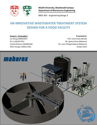
AN INNOVATIVE WASTEWATER TREATMENT SYSTEM
DESIGN FOR A FOOD FACILITY
Group 4 – AiroLeaders
Jun Dong (260442997)
Zhi Li (260331791)
Erbolat Riskulov (260483038)
Dillon Stanger (260411556)
Presented to:
Prof. Grant Clark (McGill)
Mr. Ignacio Riera (Mabarex)
Mr. Jean-Philippe Raboud (Mabarex)
18 April 2014
McGill University, MacDonald Campus
Department of Bioresource Engineering
BREE 495 – Engineering Design 3

Executive Summary
An innovative wastewater treatment system was designed for an un-disclosed slaughterhouse in Montreal for
the reduction of organics, nutrients, lipids and suspended solids while producing renewable energy.
Furthermore, this design profits 200 000 $ per year from valorising recovered nutrients rather than eliminating
them at cost as normal wastewater treatment plants do. The system components include a dissolved air
floatation unit, a dual-cycle sequencing batch reactor, an anaerobic sludge digester, and two struvite
precipitators. The design is reviewed by two professional wastewater engineers from our client Mabarex Inc.
Table of Contents
Executive Summary....................................................1
Abbreviations.............................................................2
Introduction...............................................................3
Problem Statement ............................................... 3
Objectives .............................................................. 3
Analysis and Specifications.........................................3
Treatment System ................................................. 3
DAF Unit................................................................. 4
Dual-Cycle SBR....................................................... 6
SBR Mixing and Aeration..................................... 12
SBR pH Control..................................................... 14
Anaerobic Sludge Digester .................................. 14
Centrifuge............................................................ 17
Struvite Precipitator ............................................ 18
Pumping............................................................... 20
Simulation and Optimisation....................................21
Influent ................................................................ 22
DAF Unit .............................................................. 22
Dual-Cycle SBR..................................................... 23
SBR Mixing and Aeration..................................... 27
SBR pH Control .................................................... 27
Anaerobic Sludge Digester .................................. 28
Centrifuge............................................................ 28
Struvite Precipitator............................................ 29
Testing and Optimisation.................................... 30
Safety and Economics.............................................. 31
Environmental Safety.......................................... 31
Occupational Health and Safety.......................... 32
Economics............................................................ 32
Conclusion............................................................... 33
Design Paper Competition .................................. 34
Acknowledgements............................................. 34
References............................................................... 35
1

Abbreviations
Actual oxygen transfer rate AOTR
Bio-soluble chemical oxygen demand bsCOD
Chemical oxygen demand COD
Day(s) d
Dissolved air floatation DAF
Dissolved oxygen DO
Fat, oil and grease FOG
Flow rate Q
Hour(s) h
Mean hydraulic retention time HRT
Nitrogen N
Nitrogen in form of ammonium N-NH4
Nitrogen in form of nitrate N-NO3
Non-soluble chemical oxygen demand nsCOD
Phosphorus P
Phosphorus in forms of phosphates P-PO4
Safety factor SF
Sequencing batch reactor SBR
Soluble chemical oxygen demand sCOD
Standard oxygen transfer efficiency SOTE
Standard oxygen transfer rate SOTR
Sulfur S
Sulfur in form of hydrogen sulfide S-H2S
Sulfur in form of sulfate S-SO4
Temperature T
Total Kjeldhal nitrogen TKN
Visual basic for applications VBA
Volatile suspended solids VSS
2

Introduction
Problem Statement
Due to the new stringent bylaw from the Montreal
Metropolitan Community concerning industrial
wastewater discharging into the municipal sewage,
a food processing facility (confidential) in Montreal
is required to implement a wastewater treatment
system for its three effluents. These three
wastewater streams are combined into one inside an
equalisation tank providing a stable wastewater flow
of 113 m3/d. The wastewater conditions and the
bylaw limits (CMM, 2008) are listed in Table 1:
Table 1. Wastewater conditions and bylaw limits
Criteria Wastewater Bylaw
Q (m3 d-1) 113 N/A
COD (g m-3) 7804 800
TKN (g m-3) 2063 70
N-NH4 (g m-3) 1530 45
P-PO4 (g m-3) 66 20
S-H2S (g m-3) 13 5
FOG (g m-3) 661 250
VSS (g m-3) 417 500
T (oC) 68 65
pH 6.7 6.0 – 11.5
The COD is an indication of organics content in water.
The COD characteristics are covered in Table 2.
Table 2. COD characteristics
sCOD/COD 37%
bsCOD/COD 32%
nsCOD/COD 63%
The NTK is the total nitrogen in forms of ammonium
(NH4
+) and proteins in the wastewater. The
phosphorus exists as orthophosphate (PO4
3-) and
polyphosphates (PO4
-)n. The sulfur is regarded as
sulfide species that are biologically and chemically
convertible into hydrogen sulfide. The FOG
represents the total lipids in water and, finally, the
primary VSS are mainly fine meat particles, which are
made of COD, TKN, P, S and FOG, suspended in the
wastewater.
The food factory sought a solution to the problem
from our client Mabarex Inc., an engineering
consulting firm located in Montreal, specialized in
wastewater treatment. Graciously, our mentors,
Ignacio Riera, Eng., M. Eng. and Jean-Philippe
Raboud, Eng., Ph.D., from our client Mabarex
provided us with this problem for a design study.
Objectives
The primary objective of this project is to design a
wastewater treatment system able reduce
contaminants below their bylaw limits. As an
additional challenge to the problem, the
slaughterhouse is interested to recover and valorise
the wastes and nutrients (N and P) from the
wastewater treatment.
Analysis and Specifications
This analysis section will firstly present the system
process schematic with description in broad terms.
Next, mathematical models and equations will be
explained for specifying and designing every system
component. The system components were
preliminarily specified in writing or in drawings in
millimetre unit. Details concerning design,
simulation, and optimisation will be presented in the
section of Simulation and Optimisation.
Treatment System
The design of the treatment process or system
(Figure 1) was limited to: (1) to ensure that all the
contaminants are treated below their bylaw limits,
(2) to recover as much as possible the nutrients (N
and P) from the water and valorise them as fertilisers
in order to improve the operational economy, and (3)
to consider for some of the environmental and
safety issues.
3

Figure 1. The components are shown in the blue colored blocks and the arrow lines represent the water flow
and the interactions between the components
As seen from Figure 1, the combined wastewater
streams are pumped from the flow equalization tank
at the rate of 113 m3 d-1. The combined flow travels
through the DAF unit to begin the physical removal
of non-soluble contaminants. These contaminants
include most of the FOG and the VSS along with
some other constituent contaminants (such as COD,
TKN, P, and S). The wastewater then flows from the
DAF to the dual-cycle SBR to perform an anoxic cycle
and an aerobic cycle activated sludge (biological or
microbial) treatment processes. In simple terms, the
anoxic cycle is designed to isolate the soluble
ammonium and phosphate in water. The nutrients
from the anoxic effluent is then pumped to the
chemical precipitator (CHEM from Figure 1) for
recovery in form of struvite, which is a natural
mineral fertilizer that contains ammonium,
phosphate and magnesium (details about struvite on
page 31). At the same time, the sludge from the DAF
and the SBR are sent to the anaerobic sludge
digester for three purposes. Firstly, it biologically
converts the carbon content from the sludge into
around 65% of collectable methane as a renewable
energy source and 30% carbon dioxide
(Tchobanoglous et al., 2003). This method emits less
methane, a strong greenhouse gas, than the landfill
disposal of sludge. Secondly, the digestion produces
biosolids from the digested sludge remains as a
fertilizer. The biosolids suspended in the liquid is
then physically separated by a centrifuge (CENT from
Figure 1) following the digester. Thirdly, the
digestion of sludge releases more N and P into the
liquid so that extra nutrients will be recovered in the
struvite precipitator. After the nutrient recovery, the
supernatant fluid that contains some residual
contaminants (bsCOD, TKN, P-PO4, H2S, FOG and VSS)
is returned to the SBR for the second aerobic cycle
treatment before the final effluent is discharged.
DAF Unit
This project specified to select a pre-fabricated DAF
unit from a supplier named Piedmont Technical
Services or P-TEC. P-TEC designed their DAF unit with
standard volumes based on a standard HRT of
4

treatment. Therefore, the DAF unit was selected by
the flow rate as defined in Eq. 1
Flow rate is related to volume and HRT as:
𝑄𝑄 =
𝑉𝑉
𝐻𝐻𝐻𝐻𝐻𝐻
(1)
where
Q = wastewater flow rate (m3
d-1
)
V = volume (m3
)
HRT = mean hydraulic retention time, (d)
Based on the flow rate, the P-TEC MicroDAF 36-42
model (P-TEC, 2014), which is shown in Figure 2 and
Figure 3, was chosen to be the DAF unit. Moreover,
the air pressure for the DAF process is specified with
the air-to-solid (A-S ratio) equation defined in Eq. 2
(Tchobanoglous et al., 2003). For the optimal non-
soluble contaminant removals, a DAF unit from
slaughterhouses was recommended to specify an A-
S ratio of 0.03 L g-1 (De Nardi, 2008), resulting an
operational air pressure of 4 atm. This pressure will
ensure the generation of adequately sized micro-
bubbles that attach to the VSS particles in the
wastewater and lift them along with the FOG to the
top of the DAF unit where they will be skimmed off.
The air-to-solid ratio is defined as:
𝐴𝐴
𝑆𝑆
=
1.3𝑠𝑠𝑎𝑎(𝑓𝑓𝑓𝑓 − 1)
𝑆𝑆
(2)
where
𝐴𝐴
𝑆𝑆
= Air to solid ratio (L g-1
)
𝑠𝑠𝑎𝑎 = air solubility in water (mL L-1
)
P = pressure (atm)
𝑓𝑓 = dissolved air fraction at P (typically 0.5)
S = influent VSS concentration (mg L-1
)
Figure 2. Drawing of the DAF unit with important axial dimensions of extremity (by Erbolat Riskulov)
5

Figure 3. Illustration of the supplied P-TEC MicroDAF 36-42 (by Erbolat Riskulov and Jun Dong)
Dual-Cycle SBR
The dual-cycle SBR, as mentioned in the Treatment
System section on page 4, was specifically designed
to run two cycles. The reason for the dual-cycle
design was to be able to extract the rich amount of
ammonium dissolved in the water before it is
eliminated. The ammonium cannot be precipitated
before the SBR along with other contaminants such
as the bsCOD, VSS and FOG because these
contaminants can introduce impurities (suspended
solids) into the precipitated struvite and damage the
equipment. Consequently, an anoxic cycle (Figure 4)
was designed as the treatment cycle of the SBR to
remove those unwanted contaminants.
Figure 4. An illustration of the anoxic cycle processes,
which are the anoxic fill, the anoxic reaction, the
settling and the discharge (decant), presented in the
order from left to right (by Jun Dong).
6

Upon the completion of the anoxic cycle, most of the
effluent with high NH4
+ and PO4
3- contents is slowly
pumped to the struvite precipitator where it is
combined with the effluent coming from the
anaerobic sludge digester that also contains some
concentrated NH4
+, PO4
3- and some residual bsCOD
that the precipitator can handle (Bowers, 2007).
However, due to the streams combination, the
bsCOD from the anaerobic effluent is diluted by the
anoxic effluent so that the precipitation condition is
improved. After the NH4
+ and PO4
3- are recovered
from the struvite precipitator, the supernatant with
the diluted bsCOD and residual ammonium and
phosphate are returned to the SBR. Thus, the
returned supernatant is contaminated with the
remaining untreated TKN, P-PO4 and S-H2S by the
sludge left from the anoxic cycle (the decant stage
from Figure 4). Consequently, these contaminants
will be practically treated with an aerobic activated
sludge process that is shown in Figure 5 (Sharma,
2010; Tchobanoglous et al., 2003).
Figure 5. An illustration of the aerobic cycle
processes including the aerobic fill, the aerobic
reaction, the settling and the discharge presented in
the order from left to right (by Jun Dong).
Figure 6 below is an illustration of the interactions
between the SBR processes and the contaminants
for specifications. Inside a single SBR compartment,
the first anoxic denitrification process starts since
the anoxic fill stage where the influent is pumped in
and stirred with the denitrifiers specified at 3000 g
VSS m-3 within the sludge under an average anoxic
condition of 0.25 g DO m-3 (Tchobanoglous et al.,
2003). When the reactor is filled, the inflow will be
driven to another compartment, whereas the filled
compartment is now into the reaction stage where
the denitrification is continued.
Figure 6. The biological, chemical and physical processes within the SBR interact with the contaminants. Each of
the process is color-coded with a corresponding mathematical model. The microorganisms can practically
survive in the SBR switching between the anoxic and the aerobic conditions (by Jun Dong).
7

The denitrifiers thrive in the presence of nitrate
(electron acceptor) and bsCOD organics (electron
donor and carbon source) while being inhibited by
the increasing amount of DO. As such, the biokinetics
of denitrifiers at 20oC are governed by Eq. 3
(Tchobanoglous et al., 2003). This mathematical
model simulated the minimum denitrification
process timing, the sludge production, and the
bsCOD, N-NO3, and P-PO4 concentrations from the
anoxic effluent.
The Monod equation for denitrificant biokinetics:
𝜕𝜕𝑋𝑋𝐷𝐷𝐷𝐷
𝜕𝜕𝜕𝜕
= 𝑋𝑋𝐷𝐷𝐷𝐷 ��
𝜇𝜇 𝑚𝑚,𝐷𝐷𝐷𝐷 𝑁𝑁𝑂𝑂3
𝐾𝐾𝐷𝐷𝐷𝐷 + 𝑁𝑁𝑂𝑂3
� �
𝑆𝑆
𝐾𝐾𝐷𝐷𝐷𝐷,𝑆𝑆 + 𝑆𝑆
� �
𝐾𝐾𝑂𝑂′
𝐾𝐾𝑂𝑂′ + 𝐷𝐷𝐷𝐷
� − 𝑘𝑘𝑑𝑑𝑑𝑑𝑑𝑑� (3a)
𝜕𝜕𝜕𝜕𝑂𝑂3
𝜕𝜕𝜕𝜕
= −𝑋𝑋𝐷𝐷𝐷𝐷(𝑆𝑆𝑆𝑆𝑆𝑆𝑆𝑆) (3b)
𝜕𝜕𝜕𝜕
𝜕𝜕𝜕𝜕
= − �
1
𝑌𝑌𝐷𝐷𝐷𝐷
�
𝜕𝜕𝑋𝑋𝐷𝐷𝐷𝐷
𝜕𝜕𝜕𝜕 (3c)
where
XDN = denitrifiers concentration (g VSS m-3
)
t = time (d)
µm,DN = maximum denitrifiers specific growth rate (3.2 d-1
)
NO3 = nitrate nitrogen concentration (g N-NO3 m-3
)
KDN = denitrifiers nitrate half-rate constant (0.1 g NO3
-
m-3
)
S = substrate concentration (g bsCOD m-3
)
KDN,S = denitrifiers substrate half-rate constant (9 g S m-3
)
KO’ = DO inhibition concentration (0.11 g DO m-3
)
DO = denitrification dissolved oxygen (0.25 g DO m-3
)
kdDN = denitrifiers death rate (0.15 g VSS g-1
VSS d-1
)
SDNR = specific denitrification rate (g N-NO3 g-1
VSS d-1
)
YDN = denitrifiers yield on bsCOD (0.4 g VSS g-1
bsCOD)
From Eq. 3, the specific denitrification rate (SDNR)
varies with the food-to-microorganism ratio (F/M)
that is defined by Eq. 4 (Tchobanoglous et al., 2003).
The food-to-microorganism ratio is defined as:
𝐹𝐹
𝑀𝑀
=
𝑄𝑄𝑆𝑆𝑜𝑜
𝑉𝑉𝑋𝑋𝑉𝑉𝑉𝑉𝑉𝑉
(4)
where
F/M = food-to-microorganism ratio (g bsCOD g-1
VSS d-1
)
d-1
)
So = initial substrate concentration (g bsCOD m-3
)
V = reactor volume (m3
)
XVSS = microbial concentration (g VSS m-3
)
For the aerobic process, the returned supernatant is
mixed aerobically with the aerobes from the sludge
and the contaminant treatments begin. Two groups
of aerobes are performing the second aerobic
treatment. Referred to Figure 6, the first group is the
heterotrophs and it is responsible for the biological
oxidation of bsCOD carbons and the bio-assimilation
of TKN and P-PO4. The growth rate for heterotrophs
relies on the substrate or bsCOD level, yet the
growth is insensible to the DO levels afforded by the
standard aerations. Hence, the heterotrophic
biokinetics at 20oC are described by Eq. 5 (Riera,
2013; Tchobanoglous et al., 2003). This model
simulated the aeration timing, the removals of
bsCOD, TKN and P, and the sludge production.
The Monod equation for heterotrophic biokinetics:
𝜕𝜕𝑋𝑋𝑆𝑆
𝜕𝜕𝜕𝜕
= 𝑋𝑋𝑆𝑆 �
𝜇𝜇 𝑚𝑚,𝑠𝑠 𝑆𝑆
𝐾𝐾𝑠𝑠 + 𝑆𝑆
− 𝑘𝑘𝑑𝑑𝑑𝑑� (5a)
𝜕𝜕𝜕𝜕
𝜕𝜕𝜕𝜕
= − �
1
𝑌𝑌𝑠𝑠
�
𝜕𝜕𝑋𝑋𝑆𝑆
𝜕𝜕𝜕𝜕 (5b)
𝑑𝑑𝑑𝑑
𝑑𝑑𝑑𝑑
= −𝑛𝑛
𝑑𝑑𝑋𝑋𝑆𝑆
𝑑𝑑𝑑𝑑 (5c)
where
XS = heterotrophs concentration (g VSS m-3
)
t = time (d)
µm,S = maximum heterotrophs specific growth rate (6.0 d-1
)
S = substrate concentration (g bsCOD m-3
)
KS = heterotrophs half-rate constant (20 g bsCOD m-3
)
kdS = heterotrophs death rate (0.12 g VSS g-1
VSS d-1
)
YS = heterotrophs yield on bsCOD (0.4 g VSS g-1
bsCOD)
N = TKN cencentration (g N m-3
)
n = nitrogen assimilation ratio (0.12 g TKN g-1
VSS)
Another group of the aerobes, from Figure 6, is the
nitrifiers. The nitrifiers are mostly chemoautotrophs,
meaning that they use ammonium as their energy
source while fixing carbon dioxide for their carbon
and oxygen sources. The carbon dioxide is brought
by the aeration that is correlated to the DO level.
Besides, recall from Figure 6 that denitrification
requires nitrate. That nitrate is produced here in the
aerobic cycle after the ammonium is biologically
8

oxidized by the nitrifiers. As such, the biokinetics of
the nitrifiers at 20oC are modeled as Eq. 6
(Tchobanoglous et al., 2003). The nitrifying bio-
kinetics simulated the aeration timing, the TKN
removal and the sludge production.
The Monod equation for nitrifying biokinetics:
𝜕𝜕𝑋𝑋𝑁𝑁
𝜕𝜕𝜕𝜕
= 𝑋𝑋𝑁𝑁 ��
𝜇𝜇 𝑚𝑚,𝑁𝑁 𝑁𝑁
𝐾𝐾𝑁𝑁 + 𝑁𝑁
� �
𝐷𝐷𝐷𝐷
𝐾𝐾𝑂𝑂 + 𝐷𝐷𝐷𝐷
� − 𝑘𝑘𝑑𝑑𝑑𝑑� (6a)
𝜕𝜕𝜕𝜕
𝜕𝜕𝜕𝜕
= − �
1
𝑌𝑌𝑁𝑁
�
𝜕𝜕𝑋𝑋𝑁𝑁
𝜕𝜕𝜕𝜕 (6b)
where
XN = nitrifiers concentration (g VSS m-3
)
t = time (d)
µm,N = maximum nitrifiers specific growth rate (0.75 d-1
)
N = TKN concentration (g N m-3
)
KN = nitrifiers TKN half-rate constant (0.74 g N m-3
)
DO = dissolved oxygen concentration (3 g DO m-3
)
KO = nitrifiers DO half-saturation constant (0.5 g DO m-3
)
kdN = nitrifiers death rate (0.08 g VSS g-1
VSS d-1
)
YN = nitrifiers yield on TKN (0.12 g VSS g-1
N)
Furthermore, Figure 6 shows that phosphorus is
assimilated by all group of microbes into their cell
tissue. The assimilation of P by the microbes can be
estimated by Eq. 7 (Riera, 2013).
The bio-assimilation of phosphorus by microbes:
𝑑𝑑𝑑𝑑
𝑑𝑑𝑑𝑑
= −𝑝𝑝
𝑑𝑑𝑑𝑑
𝑑𝑑𝑑𝑑 (7)
where
P = phosphorus concentration (0.02 g P m-3
)
t = time (d)
p = phosphorus assimilation ratio (g P g-1
VSS)
X = microbial concentration (g VSS m-3
)
Moreover, some of the biokinetics parameters
depend significantly on the temperature. Those
parameters can be corrected to the actual
temperature of the water during the process by Eq.
8 (Tchobanoglous et al., 2003).
Temperature correction of different reaction rates:
𝑘𝑘𝑇𝑇 = 𝑘𝑘20 𝜃𝜃 𝑇𝑇−20℃
(8)
where
kT = temperature corrected reaction rate (g g-1
d-1
)
k20 = standard reaction rate at 20o
C (g g-1
d-1
)
𝜃𝜃 = temperature coefficient (unitless)
T = actual temperature (o
C)
In addition, during the aerobic process, the S-H2S is
chemically oxidized into S-SO4. The hydrogen sulfide
oxidation kinetics modeled for a SBR at 20oC is
presented in Eq. 9 (Sharma, 2010) for simulating the
aeration timing and the final S-H2S level.
The Monod hydrogen sulfide oxidation kinetics:
𝑑𝑑�𝑆𝑆𝐻𝐻2 𝑆𝑆�
𝑑𝑑𝑑𝑑
= −𝑘𝑘�𝑆𝑆𝐻𝐻2 𝑆𝑆�
𝛼𝛼
�
𝐷𝐷𝐷𝐷
𝐾𝐾𝑜𝑜 + 𝐷𝐷𝐷𝐷
� (9)
where
�𝑆𝑆𝐻𝐻2 𝑆𝑆� = sulfur concentration as H2S (g S m-3
)
t = time (d)
k = specific oxidation rate (107 d-1
)
α = pseudo reaction order (0.56 unitless)
DO = dissolved oxygen concentration (g DO m-3
)
Ko = DO half-rate concentration (13 g DO m-3
)
After the completion of the anoxic or aerobic process,
the mixer or aerator is then turned off to allow the
sludge settling. The adopted mathematical model
describing the physical sludge settling
(Tchobanoglous et al., 2003) is presented in Eq. 10
for simulating the settling timing and the final
suspended solids concentrations.
The adopted physical sludge-settling model:
𝑑𝑑𝑋𝑋𝑉𝑉𝑉𝑉𝑉𝑉
𝑑𝑑𝑑𝑑
= −
6.5𝑋𝑋𝑉𝑉𝑉𝑉𝑉𝑉
ℎ𝑆𝑆
exp[−(0.165 + 0.00159 𝑆𝑆𝑆𝑆𝑆𝑆)𝑋𝑋𝑉𝑉𝑉𝑉𝑉𝑉] (10)
where
XVSS = suspended solids concentration (kg VSS m-3
)
t = time (h)
hs = mean settling height (m)
SVI = sludge volume index (120 mL g-1
)
Once the sludge is settled, the effluent and the
sludge are discharged simultaneously but separately.
For each of the SBR treatment cycle, all the process
timings must follow the rules stated in Eq. 11 to
9

achieve an overall continuous treatment within the
entire system. However, as the denitrification
process time might not be equal to the aerobic
process time, one of the SBR cycle will have longer
cycle time, so that the other cycle will have an extra
idling time where the SBR compartment is
completely at rest and where equipment
maintenance can be scheduled and performed.
SBR process timing rules for continuous treatment:
𝑡𝑡𝐼𝐼 + 𝑡𝑡𝐹𝐹 = 𝑡𝑡𝑅𝑅 + 𝑡𝑡𝑆𝑆 = 𝑡𝑡𝐷𝐷 (11a)
𝑡𝑡𝐴𝐴𝐴𝐴 = 𝑡𝑡𝐹𝐹 + 𝑡𝑡𝑅𝑅 (11b)
where
tI = idling time (h)
tF = fill time (h)
tR = reaction time (h)
tS = settling time (h)
tD = discharge time (h)
tAO = anoxic or aerobic process time (h)
To comply with the timing rules for a continuous
process, six SBR compartments are required. Three
of them work on the anoxic cycle with each at
different sequences (idling and fill, reaction and
settling, or decant) while the other three are working
similarly but on the aerobic cycle. The compartment
and the SBR were sized (Figure 7 and Figure 8) with
the obtained process timings (Figure 9), the water
flow rate, the sludge concentration, and the SVI.
Lastly, the flow rate of the sludge was adjusted with
the sludge production rate and the allowable
discharging time (tD), so that content remains in
equilibrium. By simulation, a 9.3 m3 d-1 of sludge
discharge flow was specified.
Figure 7. Drawing of the designed SBR with important construction dimensions (by Jun Dong)
10

Figure 8. Mabarex Inc. provides the construction of the dual-cycle hextuple compartment SBR (by Jun Dong)
Figure 9. The anoxic and the
aerobic process timings specified
for the SBR. The denitrification
time (tF,1 + tR,1) is 6.3 h and the
aerobic time (tF,2 + tR,2) is 7.4 h.
Furthermore, the difference
between the two fill times is the
idling time (tF,2 – tF,1 = tI = 1.1 h)
occurring before the anoxic cycle.
Moreover, as each cycle takes
14.1 h, the period for the SBR to
perform both cycles is 28.2 h.
11

SBR Mixing and Aeration
The TritonTM combined mixer and aerator from AIRE-
O2 Aeration Industries was chosen for the SBR as it
provides both mixing and fine-bubble aeration
functionalities for the anoxic and the aerobic cycles.
Compared to typical dispersed air diffusers and
surface aerators, the TritonTM is relatively easier to
install and maintain; also, it does not splash
microbes and odour into air, reducing occupational
risks. By practical standards, the TritonTM can be wall
mounted at a downward angle of 45o.
The selection of the TritonTM was by specifying the
mixing and aeration powers. The mixing power is
specified by Eq. 12 (Tchobanoglous et al., 2003).
The mixing power by velocity gradient:
𝑃𝑃 = 𝐺𝐺2
𝜇𝜇𝜇𝜇 (12)
where
P = mixing power (W)
G = velocity gradient (typically 200 s-1
)
µ = dynamic viscosity (N s m-2
)
V = reactor volume (m3
)
To specify the aeration power, the AOTR (Eq. 13) is
firstly calculated. It is then corrected to the SOTR by
many specified factors as stated in Eq. 14 (MDDEFP,
2001; Stenstrom et al., 2010; Tchobanoglous et al.,
2003). The SOTR is then converted by the SOTE,
which is 0.12 kg air kg-1 O2, into the air mass flow (w)
so that the standard blower power necessary for the
aeration can be determined by Eq. 15 (Riera, 2013;
Tchobanoglous et al., 2003).
The adopted AOTR equation:
𝐴𝐴𝐴𝐴𝐴𝐴𝐴𝐴 = 𝑄𝑄(𝛥𝛥𝛥𝛥) − 1.42(𝑃𝑃𝑋𝑋,𝑉𝑉𝑉𝑉𝑉𝑉) + 4.33𝑄𝑄(𝛥𝛥𝛥𝛥𝑂𝑂3) (13)
where
AOTR = actual oxygen transfer rate (g O2 d-1
)
d-1
)
ΔS = substrate consumption (g bsCOD m-3
)
PX,VSS = sludge production rate (g VSS d-1
)
ΔNO3 = nitrate yield due to nitrification (g N-NO3 m-3
)
The adopted SOTR equation:
𝐴𝐴𝐴𝐴𝐴𝐴𝐴𝐴
𝑆𝑆𝑆𝑆𝑆𝑆𝑆𝑆
= 𝛼𝛼𝜃𝜃 𝑇𝑇−20℃
�
𝛽𝛽𝐶𝐶𝑆𝑆𝑆𝑆 − 𝐶𝐶𝐿𝐿
𝐶𝐶𝑆𝑆𝑆𝑆
� (14a)
𝐶𝐶𝑆𝑆𝑆𝑆 = 𝐶𝐶𝑆𝑆𝑆𝑆 �
𝑃𝑃𝑏𝑏 + 9.78(𝐷𝐷𝐷𝐷𝐷𝐷)𝑓𝑓
101.3 𝑘𝑘𝑘𝑘𝑘𝑘
� (14b)
𝐶𝐶𝑆𝑆𝑆𝑆 = 𝐶𝐶𝑆𝑆20 �
101.3 𝑘𝑘𝑘𝑘𝑘𝑘 + 9.78(𝐷𝐷𝐷𝐷𝐷𝐷)𝑓𝑓
101.3 𝑘𝑘𝑘𝑘𝑘𝑘
� (14c)
where
AOTR = actual oxygen transfer rate (kg O2 h-1
)
SOTR = standard oxygen transfer rate (kg O2 h-1
)
𝛼𝛼 = loss correction factor (0.45 unitless)
𝜃𝜃 = temperature coefficient (1.024 unitless)
T = temperature of water (o
C)
𝛽𝛽 = oxygen saturation factor (0.95 unitless)
CSW = DO saturation in wastewater (g DO m3
)
CL = aerated liquid DO level (3.0 g DO m-3
)
CST = standard p DO saturation in water (9.08 g DO m-3
)
CSS = standard DO saturation in pure water (g m-3
)
CS20 = standard T DO saturation in water (9.09 g DO m-3
)
Pb = barometric pressure (101.3 kPa)
DWD = aeration depth (m)
f = effective depth factor (0.3 unitless)
The adopted blower power equation:
𝑃𝑃𝑤𝑤 =
𝑤𝑤𝑤𝑤𝑤𝑤
8.41𝑒𝑒
��
𝑝𝑝2
𝑝𝑝1
�
0.283
− 1� (15)
where
Pw = blower power (W)
R = ideal gas constant (8.314 J mol-1
K-1
)
T = inlet air temperature (K)
e = blower efficiency (0.65 unitless)
p2/p1 = ratio of outlet-to-inlet pressure (unitless)
The analysis specified the implementation of the
AIRE-O2 Triton 3.75 kW model (Figure 10 and Figure
11) for the SBR. The mixer motor provides 2 kW of
mixing capacity, whereas the blower provides 1.75
kW for aeration (AIRE-O2, 2014). The standard
powers are suitable with the actual values for a
safety factor of 1.2 for both the blower and the mixer.
12

Figure 10. Dimensions and mounting of the TritonTM 3.75 kW model (by Jun Dong)
Figure 11. Illustration of the supplied AIRE-O2 TritonTM 3.75 kW model (by Jun Dong)
13

SBR pH Control
During the first anoxic cycle, the denitrification of
each mole of nitrate contributes to a mole of
hydroxyl ion that shifts the pH to 10.1. The optimal
pH for denitrifiers ranges from 7.5 to 9.0 (Glass et al.,
1997), but for this project, a pH of 9.0 is specified as
it is also optimal for the nutrients recovery by
struvite precipitation, which will be recapped in the
precipitator specification section on page 18.
Furthermore, there is a deficient amount of
phosphate necessary to recover most of the
ammonium in form of struvite. Thus, phosphoric acid
at 73.2 kg H3PO4 d-1 was specified to lower the pH
while supplying phosphate as a struvite reactant
before magnesium is added in the precipitator.
Moreover, during the second aerobic cycle, every
mole of ammonium nitrified yields two hydrogen
ions that reduce the pH to 1.2. However, the
nitrifiers are suitable for a neutral pH (Riera, 2013;
Tchobanoglous et al., 2003). Therefore, a pH of 7.0
was specified for the aerobic process with the use of
sodium hydroxide. Although lime (CaCO3) is usually
applied as an economical alkalinity source, to ensure
high struvite purity, lime was suggested not to be
used throughout the treatment system as Ca3(PO4)2
will be precipitated instead. Consequently, sodium
hydroxide was chosen for its acceptable price range,
its strong base property and the purity of the struvite
that it provides. Chemical simulation specified that
288 kg NaOH d-1 should be dosed during nitrification.
Anaerobic Sludge Digester
For small anaerobic sludge digestion applications, a
contact high-rate anaerobic sludge digester was
specified for a construction design. An overview of
the anaerobic sludge digestion processes is
presented in Figure 12. The HRT inside an anaerobic
sludge digester was specified to be 10 days with 50%
sludge digestion at a controlled 35oC mesophilic
temperature (Tchobanoglous et al., 2003) for the
optimal time, space and economy efficiencies.
Figure 12. The sludge is subject to different digestion processes shown from left to right. At a controlled
temperature of 35oC, the anaerobes take from 10 to 30 days to decompose 50-66% the sludge solids into soluble
and volatile monomers. The remaining indigestible biosolids are candidate for fertilizer (by Jun Dong).
14

Therefore, the anaerobic digester volume was sized
similarly with Eq. 1 based on the 10-day HRT and the
10 m3 d-1 sludge flow rate. Furthermore, for a smaller
footprint and an adequate mixing efficiency, the
digester was specified to be a tall cylinder with a
minimum height of 6 meters (Tchobanoglous et al.,
2003). As a result, the digester was specified as 100
m3 large with 6 m height and 4.6 diameter (Figure 13
and Figure 14).
For specifying the construction material, the digester
heat loss was approximated with Eq. 17 and typical
digester material properties and thicknesses. The
simulation specified the winter conditions of -25oC
air temperature, -5oC ground temperature and 6.7 m
s-1 wind speed (Howell et al. 2009).
Heat transfer equation:
𝑞𝑞𝑙𝑙𝑙𝑙𝑙𝑙𝑙𝑙 = 𝑈𝑈𝑈𝑈(∆𝑇𝑇) (17a)
𝑈𝑈 =
1
∑
1
ℎ
+ ∑
𝑥𝑥
𝑘𝑘
(17b)
where
qloss = heat loss (W)
U = thermal conductance (W m-2
K-1
)
A = surface area (m2
)
ΔT = temperature difference (K)
h = convective heat transfer coefficient (W m-2
K-1
)
x = conductive material thickness (m)
k = thermal conductivity (W m-1
K-1
)
The construction and insulation materials include
concrete, steel and slag wool (Tchobanoglous et al.,
2003). Their thicknesses were specified and reported
in Figure 13 in millimetres.
Figure 13. Drawing of the designed anaerobic sludge digester with dimensions for construction (by Jun Dong)
15

Figure 13. Anaergia provides the manufacture of the designed anaerobic sludge digester (by Jun Dong)
The heat conductivity for the materials and the
forced convective heat transfer coefficient (Holman,
2009; Howell et al. 2009) are listed in Table 4 for heat
loss simulation. The result of heat loss is ≤ 6.4 kW.
Table 4. Heat transfer parameters
k concrete (W m-1
K-1
) 0.8
k stainless steel (W m-1
K-1
) 43
k slag wool (W m-1
K-1
) 0.038
ho, air (W m-2
K-1
) 34
The actual mixing power similarly specified by Eq. 12
is 2.85 kW. The methane produced from the
digestion, which was estimated with the following Eq.
16 (Tchobanoglous et al., 2003), has a thermal value
of 37.5 MJ m-3 CH4 (City of Palo Alto, 2007).
Estimation of methane gas generation:
𝑉𝑉̇ = 𝐺𝐺𝑜𝑜(𝑄𝑄∆𝑆𝑆 − 1.42𝑃𝑃𝑋𝑋,𝑉𝑉𝑉𝑉𝑉𝑉) (16a)
𝑃𝑃𝑋𝑋,𝑉𝑉𝑉𝑉𝑉𝑉 =
𝑄𝑄𝑄𝑄∆𝑆𝑆
1 + 𝑘𝑘𝑑𝑑(𝑆𝑆𝑆𝑆𝑆𝑆)
(16b)
where
𝑉𝑉̇ = methane generation rate (L d-1
)
Go = methane-substrate ratio (0.4 L CH4 g-1
COD)
Q = sludge flow rate (m3
d-1
)
ΔS = substrate consumption (g COD m-3
)
PVSS = anaerobes production rate (g VSS d-1
)
Y = anaerobes yield on COD (0.08 g VSS g-1
COD)
kd = anaerobes death rate (0.03 d-1
)
SRT = sludge retention time, HRT equivalent (10 d)
16

From Eq. 16, the consumed amount of substrate (ΔS)
was determined by the specific COD released from
the sludge dry mass, which is 1.42 g COD g-1 VSS,
multiplied by a typical COD utilisation efficiency of 90%
(Tchobanoglous et al., 2003). As a result, 16.8 kW of
energy was generated from 38.4 m3 d-1 of methane.
For, a 20 kW biogas boiler was specified to the
manufacturer as shown in Figure 13. Approximately
7 kW of methane heat was designed to compensate
the heat loss for keeping the digester at 35°C,
whereas the excess energy was considered to cut
other expenses from electrical heating usages in the
slaughterhouse. Moreover, during the digestion,
each gram of COD solubilised from the sludge
releases 5% of N-NH4 (Riera, 2013) and 0.5% of P-PO4
(Bowers, 2007).
Lastly, the digester typically produces carbon dioxide
at 30% of partial pressure. Consequently, the
carbonic acid is formed by the dissolved carbon
dioxide in water (Tchobanoglous et al., 2003). This
acidity shall be neutralised by the use of sodium
hydroxide. The dosage rate of sodium hydroxide was
specified to be 2.6 kg NaOH d-1.
Centrifuge
The centrifuge was specified for a digested sludge flow rate of 10 m3 d-1. The centrifuge model CS10-4 from
CENTRISYS (CENTRISYS, 2014), which is displayed in Figure 14 and Figure 15, was selected.
Figure 14. Drawing of the centrifuge with axial dimensions of extremities (by Zhi Li)
17

Figure 15. Illustration of the supplied CENTRISYS CS10-4 dewatering centrifuge (by Zhi Li and Jun Dong)
Struvite Precipitator
It is important to recall that the wastewater does not
contain enough phosphate to recover most of the
ammonium by precipitating struvite. Furthermore,
magnesium is also required to start the precipitation.
Moreover, a pH of 9.0 is required for the ionisation
of phosphate. For the cost efficiency of the reactants,
the precipitation reaction, which is represented by
Eq. 17, was specified for a pH of 9.
NH4
+
+ Mg(OH)2 + H3PO4 + NaOH + 3H2O
→ NH4MgPO4 ∙ 6H2O + Na+ (17)
However, the wastewater already contains some
dissolved phosphate. As a result, from Eq. 17, less
phosphoric acid will be dosed and the will become
greater than 9.0. To mitigate this effect, 20% molar
of the magnesium hydroxide was changed to
magnesium chloride (MgCl2) that is weakly acidic.
Therefore, the chemical concentration and dose rate
was specified as shown in Table 5.
Table 5. Reactant dose rates
Reactants Dose rates (kg d-1)
Mg(OH)2 361
MgCl2 116
H3PO4 487
NaOH 297
18

Furthermore, the mass-balanced solubility product
(Doyle and Parsons, 2002) stated in Eq. 18 solves the
amount of struvite precipitated by the desaturation
of the reactant concentrations.
𝐾𝐾𝑠𝑠𝑠𝑠 = ([𝑁𝑁𝐻𝐻4
+] − 𝑋𝑋) ([𝑃𝑃𝑂𝑂4
3−] − 𝑋𝑋) ([𝑀𝑀𝑀𝑀2+] − 𝑋𝑋) (18)
where
Ksp = struvite solubility product (4.36 × 10-13
mol3
L-3
)
[NH4
+
] = ammonium concentration (mol L-1
)
[PO4
3-
] = orthophosphate concentration (mol L-1
)
[Mg2+
] = magnesium concentration (mol L-1
)
X = struvite formation (mol L-1
)
The struvite precipitator is selected from Multiform
Harvest Inc., a supplier of our client. As found in
Figure 16 adopted from Multiform Harvest Inc., the
struvite precipitator was specified as an inverted
cone having a 4.55 m height and a 0.91 m wide on
top diameter (Bowers, 2009). Thus, each precipitator
provides a volume of one cubic meter (1 m3). A 15-
minute HRT was specified (Multiform Harvest Inc.,
2013), according to Eq. 1, two precipitators are
required to accommodate a 122.3 m3 d-1
precipitation flow while providing a 1.6 safety factor.
However, 15-minute HRT was specified only for a
conventional struvite precipitation on the post-
anaerobic stream without the addition of extra
phosphate for enhanced ammonium recovery. The
future procedure for an optimal specification will be
discussed on the Simulation and Optimization
section on page 29.
Figure 16. Drawing of the struvite precipitator with its important dimensions (by Jun Dong)
19

Figure 17. The supplied 25000 GPD struvite precipitator model from Multiform Harvest Inc. (by Jun Dong)
Pumping
The overall pumping power requirement needs to
compensate the water elevation difference (static
pressure), the flow velocity (dynamic pressure), and
the piping friction and bend losses summarized with
Eq. 19 and Eq. 20 (Crowe et al., 2009).
The pumping power is computed as:
𝑃𝑃 = 𝛾𝛾𝛾𝛾ℎ𝑝𝑝
where
P = pumping power (W)
𝛾𝛾 = fluid specific weight (N m-3
)
Q = flow rate (m3
s-1
)
hp = total pumping pressure head (m)
(19)
The head loss within piping is calculated as:
ℎ𝑝𝑝 = (𝑧𝑧2 − 𝑧𝑧1) +
𝑢𝑢2
2𝑔𝑔
�1 + � 𝐾𝐾𝐿𝐿 +
𝑓𝑓𝑓𝑓
𝐷𝐷
�
(20a)
𝑢𝑢 =
𝑄𝑄
𝜋𝜋 �
𝐷𝐷
2
�
2
(20b)
𝑓𝑓 =
64
𝑅𝑅𝑅𝑅
=
64
�
4𝑄𝑄
𝜋𝜋𝜋𝜋𝜋𝜋
�
, (𝑅𝑅𝑅𝑅 ≤ 2000 )
where
z = water elevation level (m)
u = flow velocity (m s-1
)
g = acceleration due to gravity (9.81 m s-2
)
KL = bend loss coefficient (unitless)
(20c)
20

f = friction factor (unitless)
L = pipe length (m)
D = pipe diameter (m)
Re = Reynolds number (unitless)
𝜈𝜈 = kinematic viscosity (10-6
m2
s-1
at 20o
C)
After a preliminary analysis, it was important to
notice that the flow rate is too low for a significant
flow velocity (u = 0.0013 m s-1) through any pipe.
Hence, the power to compensate the dynamic
pressure and the pressure losses become negligible
when compared to the static pressure compensation.
Moreover, the specific weight for water is 9810 N m-
3 (Crowe et al., 2009) and 10006 N m-3 is for the
sludge (Tchobanoglous et al., 2003). Three pumps
with their efficiency were chosen by selecting a
corresponding flow rate and elevation head from
their performance curve (Price Pumps, 2014). These
pumps are specified in Table 6.
Table 6. Pumping specifications
Connection Parameters Values
Equalization tank to SBR
Pump model Price RC200 1450RPM 50Hz
Pump efficiency (%) 38
Actual power (W) 28
Standard power (W) 88
SBR to precipitator
Pump model Price RC200 1750RPM 60Hz
Actual power (W) 58
SBR sludge to digester
Pump model Price LT 2900RPM 50Hz
Actual power (W) 6
Simulation and Optimisation
This section is dedicated to explain the procedures
that were went through to achieve the preliminary
specifications. As physically prototyping of the
designed system would require money and more
time to build and test, a simulation was performed
to generate the preliminary specifications. A
simulation software was created on Microsoft Excel
VBA by Jun Dong and Zhi Li for a more user-friendly
direct analysis, inverse synthesis, optimisation, and
instrumentation for the entire wastewater
treatment system. However, the modification of
calculation algorithms is more difficult compared to
its spreadsheet counterpart. Moreover,
computational models are developed on MATLAB
SimulinkTM by Jun Dong and Dillon Stanger to
synthesize all the SBR process timings. These
simulations will be explained in the following
subsections. In addition, the KTH Visual-MINTEQ 3.1
beta chemical simulation software was used for
analysing different chemical equilibria such as for
the pH controls and the precipitation of struvite.
The preliminary specifications were generated by
the simulations. The simulated results were
optimised by carrying out several iterations thereby
resulting optimised steady-state specifications.
Therefore, the simulation and the optimisation are
combined into this one section.
21

Influent
The influent tab from the VBA software (Figure 18)
had provided a direct analysis of the combined
influents flow rate and contaminant concentrations.
These values then specified, simulated and
optimised the system components. The combined
influent concentrations were computed by mass
balance (Eq. 21).
Mass balance of solute in solvent:
𝐶𝐶𝐶𝐶 𝑄𝑄𝐶𝐶 = � 𝐶𝐶𝑖𝑖 𝑄𝑄𝑖𝑖
3
𝑖𝑖=1
(21)
where
Cc = combined concentration (g m-3
)
QC = combined flow rate (m3
d-1
)
i = influent number (unitless)
Ci = concentration of an influent (g m-3
)
Qi = flow rate an influent (m3
d-1
)
Figure 18. The blue fields show the input conditions for the original three waste streams. The white fields, which
are locked for any unattended modification, are the result of the analysis.
DAF Unit
Referred to Figure 19, the flow rate specified an
appropriate DAF unit from the P-TEC MicroDAF
series. The specified A-S ratio and the air solubility or
sa (Tchobanoglous et al., 2003) determined the
minimum operational air pressure. Moreover, the
percent mass contaminant removal was entered.
Although these removal values were adopted from a
slaughterhouse DAF case study (Massé and Masse,
2000), a pilot scale chemical analysis on the primary
sludge can provide specific values. A 20oC water
temperature was assumed after the equalisation
tank (Riera, 2014). Lastly, the contaminant removals,
the DAF effluent conditions, and the primary sludge
flow rate to the digester were computed.
22

Figure 19. The fields highlighted in blue were filled at once and the white fields automatically displayed
important values for analysis and design of the next SBR and the later anaerobic sludge digester.
Dual-Cycle SBR
From the Initial Conditions (Figure 20), the dilution
of influent contaminants by the remaining sludge
liquid was computed. Furthermore, some of the
Design Conditions were specified and the Biokinetics
were corrected to the F/M ratio and the
temperature. Next, the Anoxic and Aerobic
Parameters were input to the computational Monod
biokinetics models built on MATLAB SimulinkTM as
shown from Figure 21 and Figure 22. The simulation
then returned the results seen from Figure 23 and
Figure 24. These results were entered back to the
VBA simulator (the blue fields) for iterating the
average sludge production and flow rate, the
equilibrium sludge concentration, and the sludge
concentration for settling. The sludge concentration
was then transferred to the settling model in Figure
25. After the settling simulation, the settling time
obtained (Figure 26) was then cited to the VBA
simulator for synthesising the process timings and
the SBR volumes that are respectively shown in the
frames of SBR Process Design and Hextuple SBR
Sizing from Figure 20. This process was repeated
several times until the optimised steady state values
were obtained. The final effluent pollutants were
below the limits. The hextuple compartment design
of the SBR was suggested by Mabarex Inc. (Riera,
2014) to save construction material. Maberex Inc.
also specified a 100 mm wall thickness (Riera, 2014).
Additionally, the central hexagonal island side length
of 1.5m was optimised for accommodating the mixer
and aerator plus some standing space. The 2m SBR
height was optimised for an acceptable settling time,
also for the mixer impeller and the aerator diffuser
reaching the lowest water level.
23

Figure 20. Values from the Parameters and from part of the SBR Process Design frames prepare inputs for the
SimulinkTM simulation. The remaining blue fields for input are mostly for the SimulinkTM simulation results,
whereas the remaining white fields show the SBR specifications and the effluent conditions.
Figure 21. The SimulinkTM computational model of Eq. 3 and Eq. 7 simulated the anoxic treatment process. The
blue blocks indicate where the values from the VBA simulator should be entered.
24

Figure 22. The SimulinkTM computational model for simulating the aerobic treatment process; the blue blocks
indicate where the values from the VBA simulator should be entered.
Figure 24. The anoxic timing was obtained from the left graph when the bsCOD (green line) and the N-NO3
(blue line) converged to 0 g m-3. The final denitrifier concentration was obtained from the right side graph.
25

Figure 24. The aerobic timing was obtained from the left graph when the TKN (yellow), bsCOD (green), and the
H2S (red) converged to 0 g m-3. The final aerobe concentrations were obtained from the right side graph.
Figure 25. The SimulinkTM computational model for simulating the sludge settling; the blue blocks indicate where
the values from the VBA simulator should be entered.
Figure 26. The sludge settling times for the anoxic cycle (left) and the aerobic cycle (right) were obtained when
their sludge concentration drops to 0 kg m-3.
26

SBR Mixing and Aeration
The AOTR required for the biological treatments (9
kg O2 h-1) was automatically optimised by the SBR
iteration for steady-state specification. However,
due to the wastewater impurities, a minimal 3 g DO
m-3 required a SOTR of 31 kg O2 h-1. Hence, the
blower should provide 1.43 kW of power. Moreover,
a computed minimum power of 1.72 kW should
assure an adequate mixing. Additionally, the
simulation calculated a total power consumption of
9.74 kW by the SBR as it is always operating with two
working mixers and aerators.
SBR pH Control
Referred to Figure 27, the wastewater influent with
6.7 pH was firstly balanced with the SBR sludge,
which having a pH of 7.0, left from the previous
aerobic cycle. Thus, the initial anoxic cycle pH
became 6.8. Hydroxides were produced during the
denitrification, which increased the pH to 10.1. Once
the phosphate and the hydrogen ion concentrations
are respectively balanced to 6.64E-3 mol PO4
3- L-1
and 0.007 mol H+ L-1 with H3PO4 supplements, the
dosing rate was specified. These concentrations
mean that the post-denitrification pH was lowered
to 9.0 (Figure 29). Moreover, the aeration of the
returned influent produced acids and buffering
conjugates (SO4
2-). A balanced acid concentration,
with the main buffer (SO4
2- and PO4
3-) concentrations,
simulated for a pH of 7.0 (Figure 30). The
concentration difference between the balanced and
the produced acids was the sodium hydroxide
alkalinity required for specification (Figure 28).
Figure 27. The SBR pH balance was used in conjunction with KTH Visual-MINTEQ for analysing the pH change
during the anoxic and the aerobic cycles, so that the pH controls were specified.
27

Anaerobic Sludge Digester
The simulation (Figure 31) computed the total sludge
flow from the DAF unit and the SBR into the
anaerobic sludge digester. With the specified HRT
and digester height, the digester was sized.
Furthermore, the percent sludge digestion and the
sludge composition analysed the contaminants
released into the liquid. This analysis, for optimising
the digester and the precipitator, automatically
updated every time the SBR specification is iterated.
These released contaminants calculated the
methane production and the effluent conditions.
Moreover, the structural profile was designed and
the heat loss from the digester was analysed in the
Heat Transfer frame. The heat transfer analysis
showed that the designed structural profile has
comparative heat conductance and resistance to the
conventional digesters (Tchobanoglous et al., 2003).
The heat loss accounts for about 38% heat
production from the methane. In addition, the
mixing power, which accounts for about 17% of the
methane heat production, was computed. As a result,
the digester is generating net energy at 7.6 kW.
Regarding the pH, the carbon dioxide partial
pressure and its Henry constant solved the dissolved
carbonic acid content. With the help of Visual-
MINTEQ, the amount of sodium hydroxide was
specified.
Centrifuge
The centrifuge is running at 15 kW of power while
separating 45.2 kg of biosolids per day from the
digested sludge liquid. The extracted biosolids has a
moisture content of about 60% and that dewatering
process discharges 9.8 m3 d-1 of water.
Figure 29. The simulated
results from KTH Visual-
MINTEQ showing the balanced
anoxic pH along with other
buffers at equilibrium
Figure 30. The simulated
results from KTH Visual-
MINTEQ showing the balanced
aerobic pH along with other
buffers at equilibrium
28

Figure 31. Summary of numerical inputs (blue) and results (white) for analysing and designing the digester
Struvite Precipitator
The combined flow rate, the initial concentration of
NH4
+ and PO4
3-, and the initial pH are firstly
computed from the Precipitation Parameters frame
(Figure 32). Based on the HRT, the precipitator was
specified. For the analysis, the reactive phosphate
and magnesium concentrations are specified by a
molar ratio equal to one (1). This specification must
be optimised after every iteration carried out for the
SBR to assure enough NH4
+ leaves to the SBR to
produce enough NO3
- for the SBR denitrification.
Furthermore, based on the reactive concentrations,
the desaturation concentration is inversely
simulated. The desaturation (molar removal from
Figure 32) determined that 1815 kg pf struvite could
be produced per day. The revenue from this
production is presented in the Safety and Economics
section on page 33. Moreover, the desaturation
defined the dose rate for each reactants.
However, with the specified reactant concentration
the Visual-MINTEQ, from Table 7, warned that
impurities such as magnesium phosphates would be
precipitated along with struvite. This also means that
ammonium will not be recovered as it was designed.
Table 7. Saturation of the specified precipitation
Mineral Saturation index
Mg3(PO4)2(s) 3.035
MgHPO4:3H2O(s) 0.392
Struvite 2.106
The reason is that the initial reactant concentrations,
which are shown in the Precipitation Analysis frame
from Figure 32, became too high due to the specified
reactant dose rates into the precipitator. To mitigate
the impurities, the reactant dose rates shall be
29

distributed into more precipitators, reducing the
reactant concentrations inside a single precipitator.
By doing so, the HRT will be prolonged than the one
specified by the supplier stated on page 19. This
prolonged HRT is acceptable because, as mentioned
before on page 19, the supplier did not optimised
their HRT based on the conditions of this project.
Consequently, the optimisation of implementing the
precipitators and their HRT shall be conducted using
the pilot-scaled struvite precipitator also supplied
from Multiform Harvest Inc. to our client Mabarex
Inc. The precipitation of struvite with external source
of phosphate is being studied by engineers and a
chemist from our client Mabarex Inc.
Figure 32. Summary of specifications (in blue) and results (in white) for the struvite precipitation
Testing and Optimisation
The preliminary simulation results were verified by
our mentors and compared with typical values from
the literature (Tchobanoglous et al., 2003). Three
problems were identified which related to the
denitrification process, the aeration capacity, and
the pH control. These problems, described below,
were solved and the corrected parameters were
included in the specifications presented.
The first problem was a misinterpretation on the
nitrate concentration unit for the denitrification.
Instead, the unit should be the mass of nitrogen from
the nitrate over volume (g N-NO3/m3) rather than
the mass of nitrate over volume (g NO3
-/m3). The
readjustment had been made in the simulation.
However, the simulation result showed a small 10 g
N-NO3/m3 shortage in completely removing the
bsCOD from the anoxic cycle. This problem was fixed
by adding less phosphoric acid and magnesium to
the precipitator. This modification reduced the
30

formation of struvite slightly. Thus, more ammonium
was left and then nitrified into nitrate during the
aerobic cycle for the next denitrification cycle.
Nevertheless, the simulated nitrification time did not
show a significant increase, so that the optimized
process timings and the size of the SBR were kept.
The aeration problem was that the individual blower
power of 80W was considered too low and
inaccurate by both mentors. The first cause was that
the calculation of SOTR (kg O2 h-1) did not consider
the fouling and the pressure drop effects on the air
diffuser. The second cause was that the SOTR was
not converted into airflow rate when calculating the
blower power by using the SOTE factor (it is the mass
flow of oxygen dissolved into water from the mass
flow of air). After readjustments, the preliminary
optimised aeration and mixing specifications were
simulated as stated previously on pages 12 and 27.
The last problem concerned the pH control. The
source of alkalinity was originally specified as lime
(CaCO3). However, as mentioned in SBR pH Control
on page 14, lime was replaced by sodium hydroxide
(NaOH) to avoid impurities in the struvite.
Safety and Economics
This section will discuss some of the sustainability
aspects of the designed wastewater treatment
system. These sustainability aspects include effects
on the environment, the occupational health and
safety, and the economics; the designed system
refers to the schematic in Figure 1 on page 4 and the
anticipated system setup illustrated on the cover
page. Moreover, some of the possible solutions to
those sustainability problems will be presented.
Environmental Safety
Typically, any separation of suspended solids, such
as the VSS or the sludge, from the wastewater
involves the possible use biological recalcitrant
chemical polymers or charged particles to enhance
the separation performance (Tchobanoglous et al.,
2003). Possible target system components for the
application of chemicals include the DAF unit, the
SBR and the centrifuge. However, these system
components presented above were designed not to
utilize chemicals. These components only rely on
their physical removal of suspended solids at the
costs of lower removal capacity for the DAF unit,
longer sludge settling time for the SBR, and a more
powerful centrifuge.
Only pH control and struvite precipitation utilize
chemicals. The chemicals are derivatives of natural
minerals. Furthermore, struvite (NH4MgPO4·6H2O) is
also a mineral found in nature which the authors
have not found to have any known negative
environmental impact (Westerman et al., 2009).
However, struvite crystals accumulated in animals
can eventually block their urinary tract. Thus, the
produced struvite should be stored and applied
safely so that no animal or child can ingest it. For soil
fertilisation, the release of nutrients is gradual from
the surface of struvite crystals and the release rate
can be controlled through crystal sizing. Smaller
struvite particles release more nutrients from the
first 3 to 6 weeks than the larger ones (Westerman
et al., 2009). Therefore, nutrient runoff can be
reduced. However, struvite cannot replace
conventional fertilisers as it has a fixed one-to-one
molar ratio of N and P, it lacks other nutrients such
as potassium, and it may saturate the soil with
magnesium (essential for chlorophyll synthesis in
plant growth).
One problem is that a biogas scrubber was not
specified with the anaerobic digester to remove the
volatile part of hydrogen sulfide. The combustion of
hydrogen sulfide will produce sulfur oxides that are
responsible for acid rains. For further works should
31

specify a biogas scrubber before the combustion
takes place.
Occupational Health and Safety
Railing guards are implemented to most of the
locations where falling is possible. Furthermore, the
moving parts from the most of the equipment are
covered for preventing potential injuries. The only
exception is at the center island of the SBR where the
mixer, aerator and the catwalk are mounted and
where the operator performs maintenance. The
problem there is that railing guards cannot be
installed to prevent the operator from falling into a
SBR compartment and being injured by a mixer in
operation. The reason for this problem is that the
uninstallation of mixer and aerator in case of
replacement should not be hindered and the catwalk
should be rotatable all around the SBR. Anchoring
the operator to the catwalk shall eliminate this risk
(Clark, 2014). The use of a mask is advised when
maintaining the SBR as the dissolved ammonium and
hydrogen sulfide are volatile and cause odour.
Moreover, the digester produces anaerobic compost
as biosolids fertiliser that may contain opportunistic
anaerobic pathogens. To mitigate the biohazard
from handling the biosolids, either the system shall
include a biosolids pasteurisation system using the
excess methane as its heat source, or the operator
shall be advised to use gloves, goggles and a mask.
Economics
The capital costs of the designed system (Riera, 2014;
Raboud, 2014) on this stage are listed in Table 5.
More capital expenses on the precipitators shall be
foreseen as more of them will be required.
a
(Hydro-Quebec, 2013)
b
(Parry, 2012)
c
(Wang, 2014)
d
(Yang, 2014)
Table 5. List of components and capital costs
Items Quantity Costs (CAD)
DAF Unit 1 50 000
SBR in Concrete 1 160 000
SBR Catwalk 1 30 000
SBR Aerator & Mixer 6 6 X 15 000
Anaerobic Sludge Digester 1 900 000
Centrifuge 1 320 000
Struvite Precipitator 2 2 X 85 000
Total 1 720 000
From table 5, the capital costs are high on the
digester and centrifuge. However, they are
necessary for attenuating the effect on greenhouse
gas emissions while producing more fertilisers as
addressed before.
The following Table 6 is a list of specific price in
Canadian or US dollars for consumables and goods
produced from the operation.
Table 6. List of specific prices
Item Specific Value Unit
Electricity a 0.0488 ¢ kWh-1
Biosolids b 250 $ ton-1
Mg(OH)2
c 150 $ ton-1
MgCl2
d 100 $ ton-1
H3PO4
e 700 $ ton-1
NaOH f 325 $ ton-1
Struvite g 1042 $ ton-1
The specific prices from Table 6 are multiplied by
their corresponding unit production or consumption
for determining their yearly revenue or expense
from the operation. These values are listed in Table
7.
e
(Wu, 2014)
f
(Liu, 2014)
g
(Seymour, 2009)
32

Table 7. Summary of the operational revenues, expenses and net profit
Items Quantity Revenues ($/year) Expenses ($/year)
DAF Power 9.32 kW 3 984
SBR Operating Power 9.71 kW 4 150
Anoxic pH Control 73.2 kg H3PO4/day 18 704
Aerobic pH Control 289 kg NaOH/day 34 232
Digester Mixing Power 2.85 kW 1 219
Digester pH Control 2.6 kg NaOH/day 307
Digester Net Heat Output 10.4 kW (4 447)
Centrifuge Power 15 kW 6 412
Biosolids Production 45.2 kg/day 4 126
Struvite Reactants
487 kg H3PO4/day
361 kg Mg(OH)2/day
116 kg MgCl2/day
297 kg NaOH/day
124 374
19 768
4 249
34 076
Struvite Production 1815 kg struvite/day 690 423
Pumping Power 0.3 kW 115
Wages: Manager For 1 person 70 000
Wages: Operators For 4 people 4 X 40 000
Subtotal 694 549 479 461
Pre-Tax Profit 215 088
Regarding to Table 7, the wastewater treatment
plant will need one (1) professional manager and
four (4) operators. One of the operator shall operate
the DAF unit and the centrifuge, whereas each from
the others shall operate one of the remaining
components. The salary for a wastewater treatment
plant manager and an operator are respectively
about 70 000 $ per year (Salary.com, 2014) and 40
000 $ per year (AcademicInvest.com, 2011).
In sum, the revenues were mostly from the struvite
production, whereas the expenses were mostly from
the chemicals and the wages. This wastewater
treatment system seemed having a profit potential
of 215 000 $ per year instead of deficit estimated to
be -57 000 $ per year as normal methods (such as
the DAF unit plus the SBR) do. The estimated profit
will pay the capital expenses back in a minimum of 8
years or longer if more precipitators will be needed.
Conclusion
To conclude, an innovative wastewater treatment
system was designed for the given problem and
objectives. This system includes a DAF unit, a dual-
cycle SBR, an anaerobic sludge digester, a centrifuge,
and at least two struvite precipitators. Their
preliminary specifications and analytical results were
produced through simulation and optimisations.
The designed system, reviewed by the professional
mentors, is able reduce the contaminant
concentration beyond the bylaw requirements.
Furthermore, this environmental friendly system is
able to recover nutrients dissolved in the
wastewater and to create a net profit.
33

However, before the implementation of this
innovative design, time-consuming physical pilot-
scale studies should be expensed and conducted to
validate the accuracy of the preliminary
specifications and the simulated analytical results.
For instance, the DAF unit performance must be
assessed with the actual wastewater from the
particular slaughterhouse. The effluent from the DAF
unit pilot-scale study will feed in batches a pilot-scale
single compartment SBR (instead of a hextuple-
compartment SBR for a continuous feeding) to verify
the dual-cycle SBR performance and effluent
conditions for less expense. The sludge from the DAF
unit and the pilot-scale SBR will then be continuously
sent into a downscaled anaerobic sludge digester to
determine an accurate HRT, percent digestion,
methane production, and the effluent conditions.
Finally, a single pilot-scale struvite precipitator will
determine an appropriate HRT, precipitator number,
and reactant concentrations or dose rates to
minimise the impurity in the struvite product. Once
the final specifications and results from the physical
prototyping are determined, the component
manufacturing can then be started.
Design Paper Competition
Currently, our team is participated in a design paper
competition sponsored by the Water Environment
Federation (WEF), an international organisation that
represents experts in the water engineering industry,
and by the Réseau Environnement from the province
of Quebec in Canada. The team member, Dillon
Stanger, was elected by the team to register for that
competition. The competition registration was
accepted on the week starting on the 9th of February
2014. The design competition paper can be prepared
and submitted in 3 months starting from the
submission date of this design report stated on the
cover page.
Acknowledgements
We would like to deeply and sincerely to express our
gratitude to Mr. Ignacio Riera, Mr. Carlos Sanchez
Barrios, and Mr. Jean-Philippe Raboud for spending
their precious time and resources helping our team
through this design project. Their mentorship had
brought us valuable knowledge for creating ideas
facing new challenges in the sustainability of
wastewater treatment. This honourable experience
shall be remembered. We also like to thank our
professor Dr. Grant Clark for his guidance on the
design process through his instructions, his
constructive comments and his direct answers to
questions.
Mabarex Inc.
• Ignacio Riera, Eng., M. Eng. Applications
Engineer, iriera@mabarex.com
• Carlos Sanchez Barrios, Eng., M. Sc., Project
Manager, csanchez@mabarex.com
• Jean-Philippe Raboud, Eng., Ph.D., Engineering
Director, jpraboud@mabarex.com
McGill University
• Olivier Grant Clark, Ph. D., P. Eng., Associate
Professor, grant.clark@mcgill.ca
34

References
AcademicInves.com. 2011. How to Become a Wastewater
Operator. Available at:
http://www.academicinvest.com/science-
careers/environmental-science-careers/how-to-become-a-
wastewater-operator. Accessed 21 March 2014.
AIRE-O2. 2004. AIRE-O2 Triton Process Aerator/Mixer. MN:
AIRE-O2 Aeration Industries
Anaergia. 2014. Where Some See Waste, We See Resources.
ON: Anaergia Inc.
Bowers, K. E. [Multiform Harvest Inc.]. 2007. Fluidized Bed
Crystallizer for Phosphorus Removal and Production of
Granular Struvite Fertilizer. Harvesting Clean Energy
Conference and Biodiesel in the Northwest workshop.
Idaho: DoubleTree Riverside Hotel
Bowers, K. E [Multiform Harvest Inc.]. 2009. A NEW CONCEPT
FOR REMOVAL OF PHOSPHORUS FROM DAIRY FARM
WASTE. Washington D.C.: USDA Research, Education &
Economics Information System
CENTRISYS. 2014. Centrisys Dewatering Centrifuges. WI:
CENTRISYS Co.
City of Palo Alto. 2007. Numbers, Numbers, Numbers.
Available at: http://archive.cityofpaloalto.org. Accessed:
28 February 2014
Clark, O. G. 2014. Personal conversation. Montreal, QC:
Macdonald Campus of McGill University.
Communauté métropolitaine de Montréal [CMM]. 2008.
Règlement numéro 2008-47 sur l’assainissement des eaux.
Quebec: Montreal
Crowe, C. T., D. F. Elger, Williams, B. C., J. A. Roberson. 2009.
Engineering Fluid Mechanic, 9th
Eidition. NJ: John Wiley &
Sons.
De Nardi, I. R. 2008. Performance evaluation and operating
strategies of dissolved-air flotation system treating poultry
slaughterhouse wastewater. Resources, Conservation and
Recycling, Vol.52 – Issue 3
Doyle, J. D., and S. A. Parsons. 2002. Struvite formation,
control and recovery. Water Research 36(16):3925-3940
Feedlot Services Australia [FSA]. 2002. Case Study 11 –
Dissolved Air Floatation. Queensland: FSA Environmental
Glass, C., J. Silverstein. 1997. Denitrification kinetics of high
nitrate concentration water: pH effect on inhibition and
nitrite accumulation. Water Research, Vol. 32 – Issue 3
Holman, J. P. 2009. Heat Transfer, 10th Edition. NY: McGraw-
Hill.
Howell, R. H., W. J. Coad, Sauer, H. J. 2009. Principles of
Heating, Ventilating and Air Conditioning, 6th Edition. GA:
American Society of Heating, Refrigerating and Air
Conditioning Engineers.
Hydro-Quebec. 2013. Comparison of Electricity Prices in Major
North American Cities. QC: Hydro-Quebec.
Liu, I. 2014. Competitive price wholesale Caustic Soda Flakes
NaOH. Available at: http://www.alibaba.com/product-
detail/Competitive-price-wholesale-Caustic-Soda-
Flakes_1354924843.html. Accessed 18 March 2014
Massé, D. I., L. Masse. 2000. Characterization of wastewater
from hog slaughterhouses in Eastern Canada and
evaluation of their in-plant wastewater treatment systems.
Canadian Agricultural Engineering, Vol. 42, No. 3.
Ministère du Développement durable, de l’Environnement, de
la Faune et des Parcs [MDDEFP]. 2001. Guide pour l’étude
des technologies conventionnelles de traitement des eaux
usées d’origine domestic. Quebec, QC : Gouvernement du
Québec
Multiform Harvest Inc. 2013. Designed to Meet Your Needs
with a Hassle-Free and Flexible Implementation Approach.
Seattle, WA: Multiform Harvest Inc.
Parry, D. 2012. A Look at the Economics of Biosolids. MA: CDM
Smith.
Piedmont Technical Services [P-TEC]. 2014. MicroDAF
Capacities from 12 GPM to 80 GPM. Piedmont, QC:
Piedmont Technical Services
Price Pumps. 2014. Select a Close-Coupled Centrifugal Pump.
Available at:
http://www.pricepump.com/cen_pumps.aspx. Accessed:
20 March 2014.
Riera, I. 2014. Personal communication. Montreal, QC:
Mabarex Inc.
Raboud, J.-P. 2014. Personal communication. Montreal, QC:
Mabarex Inc.
Salary.com. 2014. Waste Water Treatment Plant Manager -
U.S. National Averages. Available at:
http://www1.salary.com/Waste-Water-Treatment-Plant-
Manager-Salary.html. Accessed 21 March 2014.
35

Sharma, K. R., and Z.Yuan. 2010. Kinetics of chemical sulfide
oxidation under high dissolved oxygen levels. In SPN6,
Sixth International Conference on Sewer Processes and
Networks. Surfers Paradise, Gold Coast, Australia.
Seymour, D. 2009. Can Nutrient Recovery Be a Financially
Sustainable Development Objective? Washington D. C.:
Kennedy/Jenks Consultants.
Stenstrom, M. K., D. Rosso. 2010. Aeration. LA: University of
California
Tchobanoglous, G., F. L. Burton, Stensel, H.D [Metcalf & Eddy,
Inc.]. 2003. Wastewater Engineering – Treatment and
Reuse, 4th
Edition. NY: McGraw-Hill
Wang, J. 2014. Magnesium Hydroxide. Available at:
http://www.alibaba.com/product-
gs/202005267/Magnesium_Hydroxide.html. Accessed 23
February 2014.
Westerman, P. W., K. D. Zering, Rashash, D. 2009. Struvite
Crystallizer for Recovering Phosphorus from Lagoon and
Digester Liquid. North Carolina State University and A&T
University Cooperative Extension, 10/09—VB/KEL.
Wu, M. 2014. Phosphoric Acid. Available at:
http://www.alibaba.com/product-
gs/297192894/Phosphoric_Acid.html. Accessed 23
February 2014
Yang, A. 2014. Magnesium Chloride, Good Quality, Factory
Price. Available at: http://www.alibaba.com/product-
gs/753491128/2013_HOT_Magnesium_Chloride_good_qu
ality.html. Accessed 23 February 2014
36

SENIOR DESIGN PAPER

Recommended

Recommended

More Related Content

What's hot

What's hot (20)

Similar to SENIOR DESIGN PAPER

Similar to SENIOR DESIGN PAPER (20)

SENIOR DESIGN PAPER