GUIDELINES for SPSS STATISTICAL ANALYSES OF TESTS-1

July 2005
CNG Page 1 of 30
GUIDELINES for SPSS STATISTICAL ANALYSES OF TESTS
By Chris Green
PURPOSE:
These guidelines intend to simplify the decision-making process regarding which statistical tests
& SPSS procedures are most appropriate for various situations.
I. CLEANING DATA
The first step in any analysis is what's known as "cleaning" of data. While this might initially
sound nefarious or underhanded, it is actually a rigorous quality control check of the soundness
and credibility of the data. Any anomalies need to be clearly identified and dealt with.
Some examples of cleaning data are:
 Checking for missing data. A general Rule-of-Thumb is that no more than 5% of the total
responses should be missing. If one has large amounts of missing data some possible
causes are:
 Panelist indifference
 Lack of rigorous quality control of the Panel Coordinator
 Non-rigorous data entry standards
 Poor, confusing and/or cluttered questionnaire design
…these, and other causes, should be checked to prevent large amounts of missing data.
 Checking for numerical anomalies. For example, if a variable contains a "6" or a "0" and the
variable represents a 1-5 5-point scale, then a 6 or 0 clearly does not belong.
 Checking for unusual or unexpected distributions, or non-normal distributions. Is the data bi-
or multi-modal? If so, what statistics are appropriate, and WHY did this happen?
SPSS offers a nice quick-pass solution for initially checking data using the Explore command in
the menu:
Analyze>Descriptive Statistics>Explore
The syntax command is "Examine," and looks something like this:
EXAMINE
VARIABLES=hedonics strength appropriate
/PLOT BOXPLOT STEMLEAF HISTOGRAM
/COMPARE GROUP
/MESTIMATORS HUBER(1.339) ANDREW(1.34) HAMPEL(1.7,3.4,8.5) TUKEY(4.685)
/PERCENTILES(5,10,25,50,75,90,95) HAVERAGE
/STATISTICS DESCRIPTIVES EXTREME
/CINTERVAL 95
/MISSING LISTWISE
/NOTOTAL.
Data anomalies are situational in nature, so there is no one correct way to handle them. But it is
important that they be tracked and handled in a consistent manner.
SPSS TIP: One can always recreate menu commands via Syntax by choosing the appropriate
menu commands, then hit "Paste" instead of OK. This will open up a new Syntax window,
which you can then use to "log" repetitive menu commands.

July 2005
CNG Page 2 of 30
II. FREQUENCYand MEANS CALCULATION
First, the data file must be split by Sample
Data>Split File
Move your Sample variable into the Groups Based On window, select the Compare Groups
radio button, then click OK.
FOR SCALAR VARIABLES:
Analyze>Descriptive Statistics>Frequencies
In the Statistics box click Means in the Central Tendency Area and click Std. Deviation in the
Dispersion Area. In the Format box click Descending Values. The Syntax for this operation
looks something like this:
FREQUENCIES
VARIABLES=hedonics strength appropriate
/FORMAT=DVALUE
/STATISTICS=STDDEV MEAN
/ORDER= ANALYSIS .
SPSS TIP: Two tables will be created…to make these tables a bit more legible double-click the
means ("Statistics") table to activate it then right-click and choose the Pivoting Trays option.
Choose the Sample # (or whatever your sample variable is named) icon and drag it from Row to
Column. To clean up the Frequencies table, activate it then right-click for the Pivoting Trays.
Move the Statistics icon from Column to Layer…a Layer will now appear with a drop-down
menu…choose Valid %. Now click-and-drag your Sample % icon from Row to Column in the
Pivoting tray.
FOR MARK-ALL-THAT-APPLY DICHOTOMOUS VARIABLES:
Analyze>Tables>Tables of Frequencies
Move your dichotomous variables into the Frequencies For window. On the following buttons
choose:
 Statistics: Percents>Display
 Layout: Statistics Labels>Down the Side
 Format: Empty Cell Appearances>Zero
 Titles: Type your title here
The Syntax command looks something like this:
* Table of Frequencies.
TABLES
/FORMAT ZERO MISSING('.') /TABLES
(LABELS) > (STATISTICS) BY
( Fruity + Floral )
/STATISTICS COUNT ((F5.0) 'Count' )
CPCT ((PCT7.1) '%' ) /TITLE 'Type your title here'.
To clean up your Output table, enable the Pivoting Tray and move your Sample # variable from
Row to Column and place this above the Column icon.

July 2005
CNG Page 3 of 30
III. STATISTICAL & POST HOC TESTING
First, the data file must be unsplit by Sample
Data>Split File>Reset
Click Reset, then click OK….this will unsplit the file.
a. GENERAL RULE(S) of THUMB REGARDING CONFIDENCE LEVELS, etc:
 By convention, most data are first analyzed at the - (alpha-) risk level of =.05, which
translates to a Confidence Level (C.L.) or Confidence Interval (C.I.) = 95%*. In general, this
should be the minimum risk level that one should accept in Home-Use Tests (HUTs) or
when making decisions for picking fragrances for submissions.
 FOR EXPLORATORY or SCREENING TESTS, one may also examine at lower levels of
confidence. C.L=90% is typically looked at if post hoc tests do not yield sufficient levels or
spread amongst the samples @ C.L.=95%. One might conceivably test samples down to
the C.L.=80% level, but in no case should hypotheses be tested below this level, as one
starts to sink into the probabilistic realm of "chance." Testing at C.L.s lower than 95% are
sometimes used to prevent "throwing out the baby with the bathwater"…i.e., eliminating
potentially promising fragrances because there are insufficient differences amongst the
fragrances simply because of statistical numbers.
* Fisher RA (1956), Statistical Methodsand Scientific Inference New York: Hafner
b. SEQUENTIAL MONADIC TESTS (parametric statistics)
 Data must be entered into SPSS in a univariate manner; i.e., if there are eight fragrance
samples measured then each panelist must be represented by eight cases.
 ASSUMPTIONS:
 Observations are independent of each other;
 The data exhibit somewhat multivariate normal distribution;
 Homoscedasticity: Variances must be somewhat homogenous…SPSS prints out
Box's M and Levene's Test for Equality of Variances for this. If p<.05 then significant
differences exist between the sample variances.
 Equal sample group sizes: samples should have been evaluated a similarly equal
number of times. RULE of THUMB: Missing data should be limited to no more than
5% of the sample size, e.g., if a sample is evaluated n=100 times, then there should
be 5 or less missing answers.
i. TWO SAMPLES in SPSS (Independent-Samples T-Test):
Analyze>Compare Means>Independent-Samples T Test
1. Move scalar variable(s) of interest into Test Variable(s) window;
2. Move the Sample variable into the Grouping Variable window;
3. Define the Groups…enter the sample numbers or codes to define the Grouping
Variable;
4. Options: The Confidence Interval defaults to 95%, but you can change this here.
5. Click "OK."
The SPSS syntax used to generate this table looks like this:
GROUPS = sampleNUMBER(1 2)
/MISSING = ANALYSIS
/VARIABLES = hedonics
/CRITERIA = CI(.95) .

July 2005
CNG Page 4 of 30
i. TWO SAMPLES in SPSS (Independent-Samples T-Test): [continued]
How to read the SPSS Output:
1. Look in the Sig. Column under Levene's Test for Equality of Variances…if this number
is >.05, then one can assume that the variances are statistically equivalent.
2. Under t-test for Equality of Means: Look in the Sig. (2-tailed) column…if this number
is <.05, then there is a significant difference between the samples.
Independent Samples Test
In this case above, the Levene statistic is .679 (>.05), so we can assume equal variances. The
t-test significance is .797 (>.05), so we can assume that the hypothesis that both samples are
similarly liked is true (there is no significant difference between the samples).
ii. THREE or MORE SAMPLES IN SPSS
SPSS now allows a flexible two-way ANOVA (ANalysis Of Variance) analysis via its GLM
(General Linear Model) command. Make the following menu choices for each variable of
interest. (NOTE: The data file must be unsplit for this to work correctly.)
Analyze>General Linear Model>Univariate>
Dependent Variable: move your scalar variable of interest here
Fixed Factors: move your Sample # variable here
Random Factor(s): leave blank
Covariate(s): leave blank
WLS Weight: leave blank
Model: accept default choices
Contrasts: accept None default
Plots: not necessary…leave blank
Post Hoc: VERY IMPORTANT…move Sample # variable to Post Hoc Tests for:
Choose Sheffé, Tukey, Duncan, and Dunnett
Independent Samples Test
.172 .679 -.257 234 .797 -.076
-.257 233.771 .797 -.076
Equal variances assumed
Equal variances not
assumed
1. HEDONICS: How
much do you like or
dislike this bodyw ash
fragrance OVERALL?
F Sig.
Levene's Test for
Equality of Variances
t df Sig. (2-tailed)
Mean
Difference
t-test for Equality of M

July 2005
CNG Page 5 of 30
ii. THREE or MORE SAMPLES IN SPSS (continued)
For Dunnett accept the 2-sided radio button…choose your Control Category (i.e.,
benchmark…NOTE: your benchmark must be coded either the lowest value or highest
value of all samples for this to work correctly!)
For Equal Variances Not Assumed pick the first Tamhane's T2.
Save: leave blank
Options: you can change the default of  =.05 here…you can also select some other
diagnostics here, but your output might already be cluttered enough.
Syntaxcodeforthesecommandslookssomethinglikethis:
UNIANOVA
Liking BY Code#
/METHOD = SSTYPE(3)
/INTERCEPT = INCLUDE
/POSTHOC = Code# ( TUKEY DUNCAN SCHEFFE T2 DUNNETT(1) )
/CRITERIA = ALPHA(.05)
/DESIGN = Code# .
iii. How to Read the SPSS Output
In the left Outline Viewing pane of the Output, click onto and select Tests of Between-Subjects
Effects…this is your two-way ANOVA test. Look at Sig. In the Corrected Model row…if this
number is <.05 then you have general significance and should look at the Post Hoc results…if
not then assume no significance between the samples and go no further, even if the Post Hoc
tests indicate some significance (note: in this case below the Code # variable is related to the
Sample #).
…Inthiscase,weshouldcontinuetoexaminethePostHoctestresultstoseethespecificdifferencesbetweenthesamples.
iv. What Post Hoc tests to use, and when
There is no one "right" post hoc analysis to use, per se. The Analyst must examine the testing
situation at hand and decide which tests, or set of tests, are most appropriate. The typical level
to test at is =.05, and in most of Symrise's tests where there is no "correct" answer (unlike in a
triangle test) the test should be two-tailed. Some of the more commonly used post hoc tests
used are (listed from the most conservative, or rigorous, to the most liberal):
Tests of Betw een-Subjects Effects
Dependent Variable: Liking
555.998a 7 79.428 19.111 .000
19482.602 1 19482.602 4687.734 .000
555.998 7 79.428 19.111 .000
2460.400 592 4.156
22499.000 600
3016.398 599
Source
Corrected Model
Intercept
Code#
Error
Total
Corrected Total
Type III Sum
of Squares df Mean Square F Sig.
R Squared = .184 (Adjusted R Squared = .175)a.

July 2005
CNG Page 6 of 30
Sheffé: The most conservative…should be used only when there are a large number of
fragrance samples (at least 8), and/or when there is an unusually large n (say, over
400).
Good when there is a large spread between the highest, middle and lowest scoring
samples.
Tukey HSD (Honestly Significant Difference): Called simply Tukey in SPSS, this is a
relatively conservative test, and the most widely used amongst statisticians. A multiple
range test, it is best employed when there is a large amount of samples (6 or more).
Because of its long-standing popularity and acceptance, Tukey should probably be used
when presenting submissions to the client.
S-N-K (Student Newman-Keuls): A moderate test, in terms of conservatism.
Duncan: A modified version of the S-N-K, this test is also similar to Tukey, but more liberal.
The tests mentioned use the same equation, but Duncan and S-N-K use a lower "critical value"
than Tukey, thus are more liberal, and can create more separate significance levels between the
samples. Duncan is gaining in popularity, and can be a good test to use for developmental or
screening tests.
Fisher's LSD (Least Significant Difference): The most liberal of post hoc tests, it is most
appropriate when one has 3 samples to compare, or when there is a relative low n<50.
Other tests:
Dunnett: Widely used in the Pharmaceutical, Medical, and Biotech industries this multiple
comparison test is used to statistically compare samples to a control sample, or benchmark. A
very appropriate test to use for tests when one is only concerned about how the samples
compare to one benchmark.
Tamhane's T2: Appropriate to use when Levene's test reveals unequal variances between the
samples.
Unequal Group Sizes (unequal n): Use LSD, Games-Howell, Dunnett's T3, Sheffé, and/or
Dunnett's C.
Unequal Variances: Use Tamhane's T2, Games-Howell, Dunnett's T3, and/or Dunnett's C.
v. How to Read Post Hocs in the SPSS Output
In the Outline pane on the left side click and select the Multiple Comparisons table…one can
read the Dunnett and Tamhane's T2 here. Asterisks (*) indicates significant differences.

July 2005
CNG Page 7 of 30
To better read Tukey HSD, Duncan, and Sheffé, click on the Liking table (or whatever
variable name you tested).
Using standard significance notation conventions, here are the following levels:
vi. On Significance Notation Conventions
Uppercase letters (e.g., "A") are used to specify @ C.L.=95%…lowercase letters (e.g., "a")
signify levels @ C.L.=90%.
Liking
75 3.95
75 4.53 4.53
75 5.25 5.25
75 6.07 6.07
75 6.16 6.16
75 6.21 6.21
75 6.44
75 6.97
.646 .376 .078 .118
75 3.95
75 4.53
75 5.25
75 6.07
75 6.16
75 6.21
75 6.44 6.44
75 6.97
.079 1.000 .313 .110
75 3.95
75 4.53 4.53
75 5.25 5.25
75 6.07 6.07
75 6.16 6.16
75 6.21 6.21
75 6.44 6.44
75 6.97
.875 .699 .082 .388
Code#
535
122
329
401
150
954
668
781
Sig.
535
122
329
401
150
954
668
781
Sig.
535
122
329
401
150
954
668
781
Sig.
Tukey HSDa,b
Duncana,b
Scheffea,b
N 1 2 3 4
Subset
Means for groups in homogeneous subsets are displayed.
Based on Type III Sum of Squares
The error term is Mean Square(Error) = 4.156.
Uses Harmonic Mean Sample Size = 75.000.a.
Alpha = .05.b.
D C B A
D
CD
BC
AB
A

July 2005
CNG Page 8 of 30
STANDARD CONVENTION: Highest level is designated with an "A." In the example above
there are four levels, so the levels are designated A, B, C and D. Samples sharing the same
letter(s) do not differ from each other, so A is similar to AB, however A is significantly higher
than BC, etc.
This convention is recommended as:
 It is widely accepted & understood;
 It is easy to comprehend, and;
 One is tracking samples by the level, so it is easy to see into what level(s) any sample
belongs.
SYMRISE CONVENTION: Symrise designates each sample as to which samples they are
different from…e.g., in the example above, the ascending coded samples would be assigned
letters as such:
122=A 150=B 329=C 401=D 535=E 668=F 781=G 954=H
…So in the above Tukey HSD example above, these codes would have the following letters
next to their mean scores in a Symrise presentation:
122 - BDFGH 150 - AE 329 - EFG 401 - AE 535 - BCDFGH 781 - ACE 954 - AE
While this notation system directly compares the samples to each other, it can be confusing as:
 One must keep track as to what letter designates each sample;
 One cannot intuitively see into what level each samples resides;
 As with Sample 329 above, one does not automatically see that it scored significantly
higher than Sample E (code 535), but significantly lower than Samples F & G (codes
668 & 781).
IV. STATISTICAL & POST HOC TESTING
vii. NONPARAMETRIC TESTS - HANDLING PREFERENCES AND RANKINGS
The data used above are "parametric" in nature, i.e., the scalar data are somewhat normally
distributed. There are times, however, when one needs to deal with ordinal data that are not
normally distributed, i.e., "nonparametric"…this happens in cases where the variables

July 2005
CNG Page 9 of 30
represent rankings for preference. These tests fall into the realm of what is known as
"Probability Theory."
There are several nonparametric tests that one can run through the
Analyze>Nonparametric Tests> command:
 Chi-Square: a probabilistic distribution for two or more samples
 Binomial: a probabilistic distribution between two samples…as in the classic "coin
toss" scenario, the default Test Proportion is .50.
For the following tests, one's data must be structured in a "multivariate" manner, i.e., each
sample will have its own variable with a ranking of 1, 2 or 3, etc., so that each panelist will be
represented by one case. [If you need to restructure your data, you can do this via the
Data>Restructure command.]
 For rankings, choose K-Related Samples, since this is a direct comparison test that
does not assume independence. Check the Friedman box, and if that statistic is <.05,
then you must continue…
 …Choose 2 Related Samples option and accept the Wilcoxon Sign test default. You
must put all possible combinations of pairs, then click OK. Your Output will tell you if
any given sample pair is significantly different from one another.
V. EXPLORATORYRESEARCH: HIERARCHICAL CLUSTER ANALYSIS & PCA
This section describes the use of what is generally known as "exploratory research."
The two major methods that we will explore are Hierarchical Cluster Analysis and
Principal Component Analysis (PCA).
For these analyses, data must first be in a form like this:

July 2005
CNG Page 10 of 30
…Generally speaking, the Symrise convention is to track the % of top-two box scores for scalar
variables and to record these in a file structured as above. The goal is to relatively characterize
each fragrance according to the various descriptive or value-based attributes. One might also
analyze mean scores, but top-two box scores tend to yield greater separation between
fragrances. For dichotomous mark-all-that-apply attributes, one needs to simply enter in the
percentage of panelists that picked that attribute.
Generally, one should not include Hedonic or Appropriateness variables in these analyses.
Certainly, any JAR scales ("Just About Right") should not be included, as they are balanced
around an ideal midpoint in its scale, and would skew results in an undesirable direction…an
example of a JAR scale is the 5-point Opinion of Strength scale, where a score of 3 represents
the ideal Just About Right score.
a. TOP-TWO & BOTTOM TWO BOX SCORES
The Top-Two and Bottom-Two "Box" scores tend to be of importance to marketers and clients,
as these scores may indicate strong polarization, either good or bad. These scores represent
the percentage of panelists who scored any given fragrance in the top two, or bottom two,
choices on a scale. Additionally, clients may also be interested in the singular Top-Box or
Bottom-Box scores at the extreme ends of the scale.
a. Hierarchical Cluster Analysis
Cluster Analysis, also called data segmentation, has a variety of goals. All relate to grouping or
segmenting a collection of objects (also called observations, individuals, cases, or data rows)

July 2005
CNG Page 11 of 30
into subsets or "clusters," such that those within each cluster are more closely related to one
another than objects assigned to different clusters. Central to all of the goals of cluster analysis
is the notion of degree of similarity (or dissimilarity) between the individual objects being
clustered.
Once you have the data in the above format, click:
Analyze>Classify>Hierarchical Cluster
…Move all of the variables that you wish to analyze into the Variable(s) field. Into the
Label Case(s) By field move your Variant or Fragrance name variable (Variant in the example
above). Accept all other defaults. For the following buttons choose:
Statistics: accept defaults and also choose Proximity Matrix
Plots: accept defaults and click Dendrogram
Method: from the drop-down menu choose Ward's Method (last choice) and accept other
defaults.
Save: accept the None default
…The Syntax for this operation looks something like this:
CLUSTER Clean Harsh Fresh Moisturizing Natural AllDay fruity floral sticky dirty powdery woody watery sweet
spicy toofruity citrusy medicinal herbal soapy bitter sour toosweet green perfumey sparkling genmild wellrounded
coolcrisp freshx energizing light refreshing modern newdiff creamy common comforting cheap heavy invigorating
familiar sharp cleanx overpowering warm pampering caring oldfash soothing rich upscale sporty moisturizingp
allfamily feminine exfoliating refreshingp agedefying energizingp ultaskin hydrating masculine antistress relaxing
childrens nourishing alldayp deodorizing antibacterial
/METHOD WARD
/MEASURE= SEUCLID
/ID=VARIANT
/PRINT SCHEDULE
/PRINT DISTANCE
/PLOT DENDROGRAM VICICLE.
a. Hierarchical Cluster Analysis [continued…]
Click onto the Dendrogram table to view something like this:

July 2005
CNG Page 12 of 30
* * * * * * H I E R A R C H I C A L C L U S T E R A N A L Y S I S * * * * * *
Dendrogram using Ward Method
Rescaled Distance Cluster Combine
C A S E 0 5 10 15 20 25
Label Num +---------+---------+---------+---------+---------+
DIAL A-B CRYSTAL BRE 2 
DIAL A-B HERBAL SPRI 3 

DIAL DAILY CARE ALOE 5 

TONE HYDRATING WILD 10 

DIAL DAILY CARE EXFO 6 

DIAL DAILY CARE LAVE 7  

TONE HYDRATING MANGO 9 

DIAL A-B TROPICAL ES 4  
DIAL DAILY CARE - VI 8  
DIAL A-B SPRING WATE 1 
…It is up to the Analyst to use her/his judgment as to how many clusters one wants to report.
Ultimately, these ten fragrances have been reduced to six clusters. But an Analyst may want to
move to the right in the Dendrogram and report only three clusters, as indicated above. These
clusters represent groups of fragrances, as the panelists have characterized them via the
various attributes.

July 2005
CNG Page 13 of 30
b. Principal Component Analysis (PCA) & "Mapping"
i. Basic Description
Principal Component Analysis (PCA) is the most common form of Factor Analysis that seeks to
"reduce" and identify latent variables into sets of "dimensions" that explain the total variance
between any variables of interest. In short, it is a way to graphically characterize fragrance
samples as to how they relate, relatively, to each other, and to any variables of interest.
In its most esoteric form, PCA, and related types of factor analyses, may be considered to be a
way to "map" various products, fragrances and attributes. It is by this "mapping" terminology
that marketers most frequently refer to PCA.
PCA involves "orthogonal rotations" that involve quite complex matrix algebra to reduce
fragrances and attribute variables into more manageable "dimensions." Due to the relatively
complex nature of the mathematical theory, it may be best to explain to laypersons (e.g.,
general marketing folks) that one is trying to "position" the fragrances amongst the attributes
into two dimensions.
A typical, simple PCA, after analysis in SPSS and subsequent transformation into Excel, might
look something like this:
Ivory Honey
Ivory Waterlily
Herbal Essences
BotanicalsIris
Herbal Essences Fruit
FusionsM ango
Herbal Essences Fruit
FusionsKumquat
Olay Complete Extra Dry
Skin with Shea
Olay Complete Normal
Skin
Olay Ohm Citrus& Ginger
Olay Ohm Jasmine &
Rose
Clean
Harsh/Chemical
Fresh
M oisturizing
Natural
Like it would last all day
-1.5
-1
-0.5
0
0.5
1
1.5
2
-1.5 -1 -0.5 0 0.5 1 1.5 2 2.5
28%ofVarianceexplained
44% of Variance explained
FACTOR ANALYSIS of P&G BODYWASHES amongst P&G USERS

July 2005
CNG Page 14 of 30
c. Principal Component Analysis (PCA) & "Mapping"
ii. A Quick Word About Matrix Algebra
As previously mentioned, PCA uses some relatively complex "matrix algebra" to reduce
fragrances and attribute variables of interest into "dimensions." Realistically, everyday we
humans live in a three-dimensional [3-D] world were we move about, to use well understood
Cartesian coordinates terminology, within X (length, or width), Y (heighth), and Z (depth)
dimensions.
"Dimensions," as defined in mathematics, must be 90°, or "orthogonal," to each other, so it is
easy to understand this 3-D, X-Y-Z, world that we live in, where X, Y, and Z are all
orthogonal to each other. However, though difficult to explain fundamentally and nearly
impossible to visualize in the real world, matrix algebra allows us to use mathematics to
create and define an infinite amount of "n-dimensions." While one might reasonably
question why one would even want to do this, matrix algebra finds wide application and
use in many fields, especially when there are a large amount of variables that we wish to
"reduce" into various dimensions so that we can better classify & categorize such
variables.
An additional problem arises, graphically, when we try to explain our 3-D (or, more
problematically, n-dimensional, mathematically) world onto a sheet of paper, or onto a
computer screen, both of which are limited to two (X & Y) dimensions [2-D].
It is for this reason that in any PCA analysis, we would wish to get a decent reduction
onto the primary (X-axis) and secondary (Y-axis) axes.
iii. USES, AND ABUSES, of PCA
This "decent reduction" is generally considered to be at least 70% of the total variance
explained, or greater. SPSS will output a table that shows each factor (dimension) and what
percent of the total variance each factor explains. Of course, since we can only practically show
two dimensions on a sheet of paper, the primary (X) and secondary (Y) factors are of most
importance to us.
A problem can arise when there is not a large amount of total variance between samples, and/or
attributes, to be explained by two dimensions. So if less than 70% of the total variances are
explained by these two X & Y axes, these two axes may not meaningfully show and explain all
of the spatial relationships between the samples and attributes. A general Rule-of-Thumb is
that:
 If 70% or more of the first two X and Y factors explain the total variance, then use PCA;
 If between 50% and 70% of the variance is explained, discussion should occur among
colleagues to determine if PCA would be meaningful to support any fragrance submission;
 If less than 50% of the variance can be explained by the first two factors in PCA, then PCA
should be abandoned as "not meaningful" (and, potentially, misleading), and another
graphical method should be used (like bar charts of means, frequencies, etc.).

July 2005
CNG Page 15 of 30
iv. PCA in SPSS
1. The raw data must first be restructured into a "multivariate" format where each fragrance
represents one case and each attribute variable represents itself…the data file should look
something like this:
 Strength, and other "JAR" variables should NOT be included, as they are improper scales
for PCA;
 In general, do not include hedonic-type variables, such as Hedonics or Appropriateness,
as they are so highly related to positive attributes that these variables just clutter the
map…remember, the goal is to spatially classify the fragrances by the attributes.
 One can use either mean scores or absolute frequencies, but it is of paramount
importance that one standard be used.
 For scalar attributes, it is conventional to use the top-two box scores.
 For mark-all-that-apply variables, use the % or absolute amount picked “yes.”
One can manually enter these numbers, or, alternately, one can reconfigure the Output
tables via the Pivot Trays then copy & paste the results into this new data file.

July 2005
CNG Page 16 of 30
iv. PCA in SPSS
2. Once the data are in the proper structure within the SPSS data file
Analyze>Data Reduction>Factor…
Variables: Move all variables of interest here (NOTE: one may wish to try several
passes excluding certain variables in order to create more overall total variance), leave
the Variant variable out of this box
Selection Variable: leave blank
Descriptives: Check Univariate Descriptives, Initial Solution, Significance Levels, and
Determinant
Extraction: Method: accept the Principal Components default, check the Scree Plot then
Extract: Number of Factors: 2…accept other defaults
Rotation: click Varimax, accept defaults, and click Loading Plot(s)
Scores: once you have accepted that your PCA is viable, click Save As Variables,
accept Method: Regression default, and click Display Factor Score Coefficient Matrix
Options: accept defaults
The syntax will look something like this:
FACTOR
/VARIABLES Clean Harsh Fresh Moisturizing Natural AllDay /MISSING LISTWISE /ANALYSIS Clean Harsh
Fresh Moisturizing Natural AllDay
/PRINT UNIVARIATE INITIAL SIG DET EXTRACTION ROTATION FSCORE
/PLOT EIGEN ROTATION
/CRITERIA MINEIGEN(1) ITERATE(25)
/EXTRACTION PC
/CRITERIA ITERATE(25)
/ROTATION VARIMAX
/SAVE REG(ALL)
/METHOD=CORRELATION .

July 2005
CNG Page 17 of 30
v. Interpretation of PCA Within SPSS
Looking at the left-side Outline Viewer of the Output, there are just four tables of interest…print
out:
 Total Variance Explained
 Scree Plot
 Rotated Component Matrix
 Component Plot of Factors 1, 2
…Looking at Total Variance Explained, make sure that your first two factors explain at least
70% of the total variance:
…Inthiscase,~81.9%ofthetotalvarianceisexplainedbythefirst(X-axis;62.655%explained)andsecond(Y-axis;19.199%explained)factors,sowemaycontinue.TheScreePlot(namedafter"scree,"whichisdebrisanddirtthataccumulatesatthebottomofcliffs,etc.)lookslikethis:
Total Variance Explained
3.759 62.655 62.655 3.759 62.655 62.655 3.397 56.611 56.611
1.152 19.199 81.854 1.152 19.199 81.854 1.515 25.243 81.854
.683 11.378 93.232
.283 4.710 97.943
.112 1.863 99.805
.012 .195 100.000
Component
1
2
3
4
5
6
Total % of Variance Cumulative % Total % of Variance Cumulative % Total % of Variance Cumulative %
Initial Eigenvalues Extraction Sums of Squared Loadings Rotation Sums of Squared Loadings
Extraction Method: Principal Component Analysis.

July 2005
CNG Page 18 of 30
v. Interpretation of PCA Within SPSS
In general, one will check for the inflection point of the Scree Curve to determine the proper
number of factors to consider…in the case above, the curve starts flattening after two factors,
so, fortunately (since our presentation will be limited to two-dimensional paper!!!), only the first
two factors are perfectly appropriate to consider.
After you put the appropriate data into Excel and manipulate it, your attributes (here, minus the
overlaid fragrance plots, which we'll get to shortly) should look roughly like this, in space:
…NOW IT'S TIME TO PUT THE RAW DATA YOU HAVE GENERATED INTO EXCEL!!!…
vi. PCA Transfer from SPSS to EXCEL
1 2 3 4 5 6
Component Number
0
1
2
3
4
Eigenvalue
Scree Plot
-1.0 -0.5 0.0 0.5 1.0
Component 1
-1.0
-0.5
0.0
0.5
1.0
Component2
Clean
Harsh
Fresh
Moisturizing
Natural
AllDay
Component Plot in Rotated Space

July 2005
CNG Page 19 of 30
Follow these steps carefully, as we are now about to "fool" Excel (a "tricky" operation):
1. Create a new Excel sheet and in cell B1 write "Factor 1", in C1 write "Factor 2"
2. From your SPSS data file, copy-&-paste your fragrance names into the cells starting in cell
A2.
3. Scroll to the extreme right of your data file in SPSS. In the previous operation, you chose to
save the scores as variables…so two new variables, FAC1_1 and FAC2_1, were
created…these are the X- and Y- Cartesian Coordinates of the fragrances. Copy-&-Paste
these values into Excel next to the fragrance names starting in cell B2.
4. Double-click onto the Rotated Component Matrix in your SPSS Output Window…the table
should look something like this:
vi. PCA Transfer from SPSS to EXCEL
5. First, copy-&-paste the attribute list from this output to the cell in Column A of Excel that is
just below the last fragrance…then copy and paste the component numbers from the
Rotated Component Matrix into the cell in Column B starting after your fragrance coordinates
(as listed in Step 3, above). Your Excel file should now look like this:
Factor 1 Factor 2
DIAL A-B SPRING WATER -1.84063 0.76484
DIAL A-B CRYSTAL BREEZE 0.18234 1.28438
DIAL A-B HERBAL SPRINGS 0.25865 -0.28581
DIAL A-B TROPICAL ESCAPE -0.90166 -0.6943
DIAL DAILY CARE ALOE - RESTORE 0.49754 -1.47553
DIAL DAILY CARE EXFOLIATING - RENEW -0.1737 0.77698
DIAL DAILY CARE LAVENDER & OATMEAL 0.91736 -1.22142
DIAL DAILY CARE - VITAMINS - NOURISHING -1.01208 -0.65734
TONE HYDRATING MANGO SPLASH 0.58417 0.33013
TONE HYDRATING WILD FLOWERS 1.488 1.17806
Clean 0.965334 0.133951
Harsh/Chemical 0.007139 -0.91903
Fresh 0.616879 0.700038
Moisturizing 0.890038 -0.10356
Natural 0.867842 0.269978
Like it would last all day 0.734092 0.279915
WE ARE NOW READY TO CREATE A PCA CHART IN EXCEL!
vii. PCA in EXCEL
Rotated Component Matrixa
.965 .134
.007 -.919
.617 .700
.890 -.104
.868 .270
.734 .280
Clean
Harsh/Chemical
Fresh
Moisturizing
Natural
Like it w ould last all day
1 2
Component
Extraction Method: Principal Component Analysis.
Rotation Method: Varimax w ith Kaiser Normalization.
Rotation converged in 3 iterations.a.

July 2005
CNG Page 20 of 30
1. In Excel, highlight the beginning of your information (excluding the first header row)…in this
case it would be cells A2:C17. Then hit the Chart Wizard icon…
2. Choose XY (Scatter) and accept the default Chart sub-type…click Next
3. Click the Series tab, highlight Series 2 and click Remove
4. For X-Values highlight data in Columns A & B (in this case A2:B17)
5. For Y-values, highlight data in Column C (in this case C2:C17)…click Next
6. For the following Tabs, following this data set, one might enter:
 Title: Chart Title: "PCA Analysis of XXX"
Value (X) Axis: "63% of Variance Explained" [round to nearest integer]
Value (Y) Axis: "19% of Variance Explained"
 Axes: accept defaults
 Gridlines: unclick Major Gridlines default
 Legend: unclick Show Legend default
 Data Labels: Show Label
…click Next and…
7. Click New Sheet and label it as you wish…click Finish
vii. PCA in EXCEL (continued)
…by assigning both Columns A & B to the X-axis (Factor 1), we have just "fooled" or "tricked"
Excel into attaching the Column A labels to the data points. The ensuing Chart will look
something like this:
DIAL A-B SPRING WATER
-1.84063
DIAL A-B CRYSTAL
BREEZE
0.18234
DIAL A-B HERBAL
SPRINGS
0.25865
DIAL A-B TROPICAL
ESCAPE -
0.90166
DIAL DAILY CARE ALOE -
RESTORE
0.49754
DIAL DAILY CARE
EXFOLIATING - RENEW
-0.1737
DIAL DAILY CARE
LAVENDER & OATMEAL
0.91736
DIAL DAILY CARE -
VITAMINS - NOURISHING
-1.01208
TONE HYDRATING
MANGO SPLASH
0.58417
TONE HYDRATING WILD
FLOWERS
1.488
Clean 0.965333633
Harsh/Chemical
0.007138979
Fresh 0.616878829
Moisturizing 0.890037567
Natural 0.86784186
Like it would last all day
0.73409217
-2
-1.5
-1
-0.5
0
0.5
1
1.5
0 2 4 6 8 10 12 14 16 18

July 2005
CNG Page 21 of 30
NOTE: THIS IS NOT WHAT YOUR FINAL CHART WILL LOOK LIKE!!!!
…We must continue to "trick" Excel…
8. Click on each data label and delete the numerical portion of each label only. The idea here
is to just have the textual label attached to each data point. We will now set things straight to
get our true final PCA Chart.
9. Right-click on the chart and select Source Data…this will bring us back to the chart set-up.
10.Click on the Series tab and reset the X Values to highlight only Column B information. Your
newly correct Chart should look something like this:
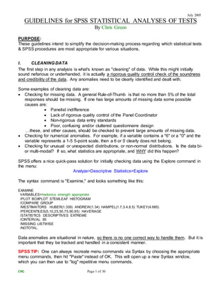
…A quick check of your Component Plot in Rotated Space (from SPSS) will reveal that your
attributes match the spaces in the chart above:
DIAL A-B SPRINGWATER
DIAL A-B CRYSTAL
BREEZE
DIAL A-B HERBAL
SPRINGS
DIAL A-B TROPICAL
ESCAPE
DIAL DAILYCARE ALOE -
RESTORE
DIAL DAILYCARE
EXFOLIATING- RENEW
DIAL DAILYCARE
LAVENDER& OATMEAL
DIAL DAILYCARE -
VITAMINS- NOURISHING
TONE HYDRATING
MANGO SPLASH
TONE HYDRATINGWILD
FLOWERS
Clean
Harsh/Chemical
Fresh
Moisturizing
NaturalLike it wouldlast all day
-2
-1.5
-1
-0.5
0
0.5
1
1.5
-2.5 -2 -1.5 -1 -0.5 0 0.5 1 1.5 2

July 2005
CNG Page 22 of 30
…TA DA!!! Besides editing your chart in Excel, you have just finished creating a PCA Chart
using both SPSS and Excel.
viii. Categorical PCA (CATPCA) ["Optimal-Scaling"]
Standard principal components analysis assumes linear relationships between numeric
variables. On the other hand, the relatively recent optimal-scaling approach allows variables to
be scaled at different levels. Categorical variables are optimally quantified in the specified
dimensionality. As a result, nonlinear relationships between variables can be modeled.
Because of this, CATPCA can be a superior & more robust (explains variances well) analysis
than standard PCA, as one is normalizing the complete raw data, as opposed to means or
top-two box scores in standard PCA. CATPCA can be particularly advantageous when
standard PCA yields insufficient results, either because the variables of interest explain little
total variance (i.e., total below 70%), or, conversely, they are so highly correlated that only one
factor explains >90% of the variance (resulting in one big cluster, with little space between the
individual variables in the cluster).
Categorical Principal Components Analysis Data Considerations
Assumptions: The data must contain at least three valid cases (which were variables before
restructuring…see below). The analysis is based on positive integer data. The discretization
option will automatically categorize a fractional-valued variable by grouping its values into
-1.0 -0.5 0.0 0.5 1.0
Component 1
-1.0
-0.5
0.0
0.5
1.0
Component2
Clean
Harsh
Fresh
Moisturizing
Natural
AllDay
Component Plot in Rotated Space

July 2005
CNG Page 23 of 30
categories with a close to "normal" distribution and will automatically convert values of string
(i.e., text) variables into positive integers. You can specify other discretization schemes.
Setting Up the Data File
The data must first be restructured & transposed, as with PCA above, so that your variables of
interest become cases (known as "objects" within CATPCA), and your cases become variables.
But unlike PCA, you will use the raw data scores. Your data file should look something like this:
CATPCA Commands in SPSS
Analyze>Data Reduction>Optimal Scaling…
Optimal Scaling Level: Some variable(s) not multiple nominal [you will see the Selected
Analysis switch to highlight CATPCA].
Number of Sets of Variables: accept the One set default…click Define…

July 2005
CNG Page 24 of 30
…move your variables-of-interest into the Analysis Variables window…highlight them in this
window and click the…
Define Scale and Weight: click on the Ordinal radio button…move the variable that
contains your variables names (now cases or "objects") into the Labeling Variables window

July 2005
CNG Page 25 of 30
…Ignore the Discretize and Missing Buttons, as you will accept their defaults…
Options: select Object Principal from the Normalization Method drop-down menu…
…Continue…

July 2005
CNG Page 26 of 30
Output: accept defaults and also choose Object scores and Variance accounted for…
…ignore Save…also ignore the Plots buttons (Object…Category…Loading…), as you will
accepts their defaults.
…The Syntax for these operations should look something like this:
CATPCA
VARIABLES=K_1 K_2 K_3 K_4 K_5 K_6 K_7 K_8 K_9 K_10 CASE_LBL
/ANALYSIS=K_1(WEIGHT=1,LEVEL=ORDI) K_2(WEIGHT=1,LEVEL=ORDI) K_3(WEIGHT=1,LEVEL=ORDI)
K_4(WEIGHT=1,LEVEL=ORDI) K_5(WEIGHT=1
,LEVEL=ORDI) K_6(WEIGHT=1,LEVEL=ORDI) K_7(WEIGHT=1,LEVEL=ORDI) K_8(WEIGHT=1,LEVEL=ORDI)
K_9(WEIGHT=1,LEVEL=ORDI)
K_10(WEIGHT=1,LEVEL=ORDI)
/MISSING=K_1(PASSIVE,MODEIMPU) K_2(PASSIVE,MODEIMPU) K_3(PASSIVE,MODEIMPU) K_4(PASSIVE,MODEIMPU)
K_5(PASSIVE,MODEIMPU)
K_6(PASSIVE,MODEIMPU) K_7(PASSIVE,MODEIMPU) K_8(PASSIVE,MODEIMPU) K_9(PASSIVE,MODEIMPU)
K_10(PASSIVE,MODEIMPU)
/DIMENSION=2
/NORMALIZATION=OPRINCIPAL
/MAXITER=100
/CRITITER=.00001
/PRINT=CORR LOADING OBJECT VAF
/PLOT=OBJECT (20) LOADING (20) .
…click OK, and now let's check out the SPSS Output.

July 2005
CNG Page 27 of 30
SPSS Output for CATPCA
The three tables that we really care about are Variance Accounted For (the Centroid Coordinate
cells highlighted above total to 97.595% explained, which is good, as it's far above our 70%
minimum criterion), Object Scores, and Casenumbers plot.
Object Scores
.188 .322
.541 -.494
.417 .431
.015 -1.121
.044 -.792
.288 .316
.367 .181
.132 .210
-.315 -.134
-.345 .221
.403 .336
.034 .099
-1.871 .129
.103 .296
Case Number
1
2
3
4
5
6
7
8
9
10
11
12
13
14
1 2
Dimension
Object Principal Normalization.

July 2005
CNG Page 28 of 30
…You will copy/paste the Object Scores coordinates into Excel, then proceed as mentioned in
the PCA section above…when finished in Excel, check and see that your Excel chart looks
something like your SPSS Object Points Labeled by Consumers chart:
-2.0 -1.5 -1.0 -0.5 0.0 0.5 1.0
Dimension 1
-1.0
-0.5
0.0
0.5
Dimension2
1
2
3
4
5
6
78
9
10
11
1213
14
Object Principal Normalization.
Object Points Labeled by Casenumbers

July 2005
CNG Page 29 of 30
VI. GENERAL SPSS TIPS, TRICKS, & TRIVIA
 SPSS stands for Statistical Program for the Social Sciences
 IMPORTING EXCEL DATA INTO SPSS:
 Prep Excel file by making sure that the first row contains Column Headers (variable
names)…save & close file
 In SPSS, File>Read Text Data>Files of Type>*.xls
 When running frequencies after splitting a data set by Sample #, SPSS reads codes in
ascending order, e.g., SPSS will list code 122 in the table before 150. It is most desirable if
SPSS lists your fragrances in the same order as in your Sample Request, so it is good
practice to create a dummy variable with recodes:
 While highlighting your Sample Code variable, click:
Data>Insert Variable
 Name this new variable something like "Sample #," etc., then copy & paste the
Sample Code data into this new variable
 Recode the new data as such 122=1, 150=2, etc.
Transform>Recode>Into Same Variables>Old and New Variables
…then put the old & new values into the respective field and click OK.
 Also, SPSS will reconfigure the order of cases in the data set after doing multiple procedures
such as Sort and Split. IT IS GOOD PRACTICE to maintain some sort of control over your
SPSS Data file so that one can compare an original SPSS file to another original file (say, an
Excel raw data file from an agency)
 Create a new dummy variable before performing any SPSS operations:
Data>Insert Variable
 Name this new variable Order, or Sorting, or something of that nature
 Examine how many cases are in your SPSS data file: e.g., 600
 Open a new Excel file and type "1" in cell A1. In Excel, select Edit>Fill>Series…click
the Columns button and set the Stop Value appropriately (e.g., 600)
 Copy-&-Paste this Excel column into your new Order column in SPSS
 Now, despite multiple Sorting and/or Splitting, one can always recall the original data
order by doing Data>Sort Cases>Sort By: Order>Ascending
 As previously mentioned one can always "clean up" and reconfigure Output tables by
selecting it and right-clicking Pivot Tables. Also:
 The left pane Outline Viewer contains a lot of "junk" so it is good practice to delete
any titles or tables that you don't need.
 One can always drag & drop tables in the Outline if you need to move tables.
 As previously mentioned, one can always recreate menu commands via Syntax by choosing
the appropriate menu commands, then hit "Paste" instead of OK. This will open up a new
Syntax window, which you can then use to "log" repetitive menu commands.
And finally…

July 2005
CNG Page 30 of 30
 …DO NOT TAUNT SPSS!!!

GUIDELINES for SPSS STATISTICAL ANALYSES OF TESTS-1

Recommended

Recommended

More Related Content

What's hot

What's hot (19)

Similar to GUIDELINES for SPSS STATISTICAL ANALYSES OF TESTS-1

Similar to GUIDELINES for SPSS STATISTICAL ANALYSES OF TESTS-1 (20)

GUIDELINES for SPSS STATISTICAL ANALYSES OF TESTS-1